4.3 Building Utilization

As seen in Section 2.10, Stockton’s population is estimated to grow from 315,000 in 2020 to 339,000 in 2040, and Stockton’s job count is estimated to grow from 125,000 in 2020 to 151,000 in 2040. The roughly 24,000 new residents and 26,000 jobs will of course have some baseline amount of energy use that can’t be avoided, but the particular ways in which buildings provide for their needs can be made more energy-efficient through specific strategies. This section will focus on ways to reduce the amount of space required per person, which primarily affects energy usage because less heating and cooling is required. Less space per person implies a more dense urban form, which also brings transportation benefits, which we account for elsewhere in the model.

4.3.1 Strategy: Accessory Dwelling Units

The 2019 California state legislative cycle resulted in accessory dwelling units (ADU) laws that took effect on 1/1/2020 and, among other changes, supercede local control to allow ADUs to be built on every single-family parcel. More specifically, local regulations cannot prevent a homeowner from applying to build an internal ADU of up to 500 sqft within their existing structure, as well as a detached ADU of up to 800 sqft in their backyard, with newly enforced maximum setbacks of 4ft from the side and rear. Exact regulatory details are still in flux as individual cities are expected to update their local ordinances to match the new state laws, and loopholes will inevitably come up; refer to CA Housing and Community Development for the latest guidance.

ADUs are being evaluated as a green economy strategy for the following key reasons.

First, internal ADUs such as garage conversions directly align with the goals of Building Utilization, making more effective use of existing built floor area and promoting less energy-intensive residential living. According to the U.S. Energy information Administration’s Residential Energy Consumption Survey (RECS 2009) (see figure below), the energy use per household in 2-4 unit dwellings is roughly half of the energy use of a single-family household, so we will use the same assumption when considering the energy impact of internal ADUs. In other words, every new internal ADU development that Stockton can enable will effectively increase household count without increasing overall energy use, assuming those households would have otherwise lived in newly built single-family homes. This liberal assumption can inform an upper-end estimate of the energy consumption benefits of internal ADUs.

include_graphics("images/energyuseduplex.png")

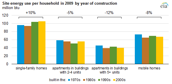
Figure 4.3: Site energy use by housing type. Source: RECS 2009.

\(~\)

Second, detached ADUs, while not as effective as internal ADUs from a building utilization perspective, still are efficient compared to the average single-family dwelling because they are likely to have a smaller footprint in the constraints of backyard development. A robust model for the relationship between square footage and energy use is outside the scope of this study, so our simplified assumption will be as follows. According to the same RECS, as analyzed by the National Association of home Builders (see figure below), about a third of single-family home energy consumption is for heating/cooling, while the rest is not significantly correlated with square footage. As previously estimated in Section 2.9, the average residential unit size in Stockton today is about 3,200 sqft (conservative because the data includes multifamily units) and consumes about 78,000 kBTUs per year. So we can estimate that a detached ADU of half that size, 1,600 sqft, would reduce its energy consumption by a sixth (to 65,000 kBTUs per year), and so forth.

include_graphics("images/nahbenergy.jpg")

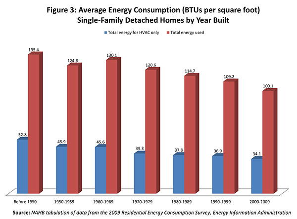
Figure 4.4: NAHB analysis of HVAC vs non-HVAC energy use. Source: RECS 2009.

\(~\)

Third, ADUs of any type can be considered “infill growth” as they do not lead to expansion of existing urban boundaries or services. Considering transportation GHGs, we can assume that a household that lives in a new ADU will have the same transportation footprint as their neighbors, where otherwise they might live in newly-built housing that is likely to be further on the outskirts of town, away from jobs and amenities. For the purposes of this section, we will conclude by demonstrating that a progressive ADU strategy could target ADU development in the areas with the least amount of car-dependence, namely transit access to downtown and other neighborhood centers.

Fourth, homeowners who develop ADUs may realize a new stream of rent revenue, building wealth for local residents, while renters may benefit from lower rents because ADUs are a form of naturally occurring affordable housing.

The fundamental question, then, is: how many new ADUs can Stockton actively enable in the next two decades that wouldn’t have otherwise been built? It is unknown what the natural rate of ADU development is without local intervention, given the new state legislation; this remains to be seen in communities across the state as the laws have just taken effect. But for the purposes of our analysis, we will assume that the City of Stockton has a range of options from being the least supportive of ADU development (given that despite state legislation, local permitting processes, permit fees, information barriers, community opposition, and financial barriers could all work to curtail development) to the most supportive of ADU development (adopting many of the best practices we reviewed in Chapter 3), and we will quantify the size of that spectrum by estimating the number of ADUs that could be built based purely on physical characteristics of existing single-family parcels.

The following is a breakdown of the number of residential parcels by housing type, based on 2018 County Assessor Records. Note that the apartment parcels contain multiple units, so the number of total housing units or households is not represented in this table. Also, our data does not clearly indicate existing ADUs, so the analysis assumes that all single family parcels do not currently have ADUs. We suspect that the existing number of permitted ADUs is relatively low.

projection <- "+proj=utm +zone=10 +ellps=GRS80 +towgs84=0,0,0,0,0,0,0 +units=ft +no_defs"

stockton_boundary_influence_projected <- st_read("C:/Users/derek/Google Drive/City Systems/Stockton Green Economy/SpheresOfInfluence/SpheresOfInfluence.shp", quiet = TRUE) %>% 
  filter(SPHERE == "STOCKTON") %>% 
  st_transform(projection)

load("C:/Users/derek/Google Drive/City Systems/Stockton Green Economy/Parcels/sjc_parcels.Rdata")

load("C:/Users/derek/Google Drive/City Systems/Stockton Green Economy/Parcels/stockton_parcels.Rdata")

load("C:/Users/derek/Google Drive/City Systems/Stockton Green Economy/USBuildingFootprints/bldg_join.Rdata")

residential_bldg <-
  bldg_join %>% 
  st_transform(projection) %>% 
  filter(ZONING == "R")

stockton_residential_parcels <-
  stockton_parcels %>%
  filter(APN %in% residential_bldg$APN) %>% 
  left_join(residential_bldg %>% st_set_geometry(NULL), by ="APN") %>% 
  filter(!duplicated(APN))

residential_bldg_summary <-
  stockton_residential_parcels %>% 
  mutate(
    Type = 
      case_when(
        type == 10 ~ "Single Family",
        type == 21 ~ "Duplex",
        type == 22 ~ "Apartment",
        is.na(type) ~ "Data Unavailable",
        TRUE ~ "Other"
      )
  ) %>% 
  group_by(Type) %>%
  summarize(Count = n()) %>% 
  st_set_geometry(NULL) %>% 
  mutate(Count = prettyNum(floor(Count/100)*100,big.mark=","))

residential_bldg_summary <- residential_bldg_summary[c(5,3,1,4,2),]

kable(
  residential_bldg_summary,
  booktabs = TRUE,
  caption = 'Number of residential parcels in Stockton by housing type.'
) %>%
  kable_styling() %>%
  scroll_box(width = "100%")

Table 4.2: Number of residential parcels in Stockton by housing type.

Type	Count
Single Family	62,200
Duplex	3,700
Apartment	400
Other	1,000
Data Unavailable	14,100

\(~\)

Starting first with internal ADUs, technically all 66,000 single-family, duplex, and apartment parcels could build permitted internal ADUs (in fact more than one can be allowed in existing multifamily buildings). These are by definition smaller units (less than 500 sqft, typically converting an existing garage, attic, basement, or master bedroom), so can’t necessarily support larger household sizes.

As projected in Section 2.10, only 25,000 new residents are expected between 2020 and 2040. In other words, it could be possible to support this entire population growth (with little increase in building energy consumption) if just half of all eligible existing buildings were to convert existing space to internal ADUs. Of course, for a number of reasons including lifestyle preference (with internal ADUs perhaps being the least palatable social arrangement for two separate households), this is not literally feasible, but should signal the opportunity in encouraging ADU development.

Detached ADUs may be more palatable (along with attached ADUs which are additions to an existing home, but these are not considered in our analysis), given the greater privacy between households, greater square footage, and potential reduced complexity of new construction vs. retrofitting existing buildings, but are more costly as well. Assessing the viability of detached ADUs is more complicated because it involves geospatial analysis.

We developed a script that performs the following basic steps:

1. We acquired Parcel shapes from the City of Stockton GIS database.
2. We acquired Building shapes from Microsoft’s U.S. Building Footprint Data
3. For each residential parcel, we produced the leftover yard area after removing 4ft setbacks, front yards (based on the closest distance from the existing building to the street edge), and the building (including a 5ft setback per municipal ordinances).
4. Using an 8ft x 20ft shape (like the smallest ADU available on the market), we traced this yard space to find the subset of space that can technically fit an orthogonal ADU design. This method does not account for obstructions like trees not represented in our data.
5. We aggregated and quantified the square footage of this remaining “buildable area”.

The following map shows what the analysis looks like for one block group in South Stockton.

# yard_setbacks <-
#   stockton_residential_parcels %>%
#   st_buffer(-4, joinStyle = "MITRE", mitreLimit = 1) # 4ft yard setback
# 
# house_setbacks <-
#   residential_bldg %>%
#   st_buffer(5, joinStyle = "MITRE", mitreLimit = 1) #5 ft house setback
# 
# adu_available_land <- NULL
# for(row in 1:floor(nrow(stockton_residential_parcels)/1000)){
# 
#   start <- row*1000-999
# 
#   end <- ifelse(
#     row < floor(nrow(stockton_residential_parcels)/1000),
#     row*1000,
#     nrow(stockton_residential_parcels)
#   )
# 
#   print(paste0(start," to ",end))
# 
#   available_land <-
#     st_difference(yard_setbacks[which(yard_setbacks$APN %in% stockton_residential_parcels$APN[start:end]),], st_union(house_setbacks[which(house_setbacks$APN %in% stockton_residential_parcels$APN[start:end]),]))
# 
#   adu_available_land <-
#     adu_available_land %>%
#     rbind(available_land)
# }
# save(adu_available_land, file = "C:/Users/derek Ouyang/Google Drive/City Systems/Stockton Green Economy/ADU/adu_available_land.Rdata")
# 
# yard_separation <- #separates front and back yards into separate shapes
#   adu_available_land %>%
#   as_Spatial() %>%
#   sp::disaggregate() %>%
#   st_as_sf()
# 
# This creates the merged parcel shapes, so you can know that a parcel touches a street edge if it shares an edge with the block it's part of. the buffers are first filling in some small slivers, and then producing an end block shape that is 1ft inset from the original.
# stockton_parcels_dissolve <-
#   stockton_parcels_extended %>% 
#   summarize() %>% 
#   st_buffer(1) %>% 
#   st_buffer(-2) %>%
#   as_Spatial() %>%
#   sp::disaggregate() %>%
#   st_as_sf()
# 
# save(stockton_parcels_dissolve, file = "C:/Users/derek Ouyang/Google Drive/City Systems/Stockton Green Economy/ADU/stockton_parcels_dissolve.Rdata")
# load("C:/Users/derek Ouyang/Google Drive/City Systems/Stockton Green Economy/ADU/stockton_parcels_dissolve.Rdata")
# 
# This creates the clips of each parcel with the block shapes from the previous line. because of the -1ft buffer, this creates little 1ft leftover crusts.
# 
# for(row in 1:floor(nrow(stockton_parcels_dissolve)/100)){
# 
# street_edges <- NULL
# for(row in 1:floor(nrow(stockton_parcels_dissolve)/100)){
#   
#   start <- row*100-99
# 
#   end <- ifelse(
#     row < floor(nrow(stockton_parcels_dissolve)/100),
#     row*100,
#     nrow(stockton_parcels_dissolve)
#   )
# 
#   print(paste0(start," to ",end))
#   
#   street_edge <- 
#     stockton_residential_parcels[which(stockton_residential_parcels$APN %in% st_centroid(stockton_residential_parcels)[stockton_parcels_dissolve[start:end,],]$APN),] %>% 
#     mutate(
#       parcel_area = st_area(.) %>% as.numeric()
#     ) %>% 
#     st_difference(st_union(stockton_parcels_dissolve[start:end,]))
#   
#   street_edges <-
#     street_edges %>% 
#     rbind(street_edge)
#   
#   save(street_edges, file = "C:/Users/derek Ouyang/Google Drive/City Systems/Stockton Green Economy/ADU/street_edges.Rdata")
# }
# 
# load("C:/Users/derek Ouyang/Google Drive/City Systems/Stockton Green Economy/ADU/street_edges.Rdata")
# 
# # Note that borders with water or green space may be incorrectly identified as street edges with this method. in EPA there are almost always buffer parcels for the baylands which prevent this from happening, but this may need to be addressed as a check on suspected throughlots using the street method, same as how the corner lot cases likely need to be sent to the street method.
# 
# # Reviewing the throughlot cases can lead to manual identification of false positives, but this may not be worth the time to do. for now, this sets aside all cases of 2+ crusts to be treated in a separate analysis, since you'd need to treat throughlots separately anyway.
# through_lots_or_misc <-
#   street_edges %>% 
#   as_Spatial() %>%
#   sp::disaggregate() %>%
#   st_as_sf() %>% 
#   group_by(APN) %>% 
#   summarize(count = n()) %>% 
#   filter(count > 1) %>% 
#   st_set_geometry(NULL) %>% 
#   left_join(stockton_parcels, by = "APN") %>% 
#   st_as_sf()
# 
# # This takes advantage of the convex hull operation to find bent crusts. 15% seems to be roughly the right ratio of the convex hull shape area to original parcel area to identify true corner conditions, but this will have some false positives and false negatives. these corner cases are set aside for now, likely need to be sent to the street matching script.
# corner_edges <-
#   street_edges %>%
#   filter(!APN %in% through_lots_or_misc$APN) %>% 
#   st_convex_hull() %>% 
#   mutate(
#     edge_area = st_area(.) %>% as.numeric()
#   ) %>% 
#   filter(edge_area > parcel_area*0.15)
# 
# This filters to the remaining one-crust parcels that are SFR. 
# normal_residential_parcels <-
#   street_edges %>% 
#   filter(!APN %in% through_lots_or_misc$APN) %>%
#   as.data.frame() %>% 
#   rename(street_edge = geometry) %>% 
#   dplyr::select(APN,parcel_area,street_edge) %>% 
#   left_join(stockton_parcels, by = "APN") %>%
#   as.data.frame() %>% 
#   rename(parcel_geometry = geometry) %>% 
#   dplyr::select(APN,parcel_area,street_edge,parcel_geometry) %>% 
#   right_join(residential_bldg, by = "APN") %>%
#   filter(!is.na(parcel_area)) %>% 
#   rename(building_geometry = WKT) %>% 
#   st_as_sf()
# 
# normal_residential_parcels_distance <-
#   normal_residential_parcels %>% 
#   mutate(
#     distance_bldg_front =
#       1:nrow(normal_residential_parcels) %>% 
#       map(function(row){
#         if(row%%100 == 0) print(row)
#         st_nearest_points(normal_residential_parcels$street_edge[row],normal_residential_parcels$building_geometry[row]) %>% 
#           st_length()
#       }) %>% 
#       unlist()
#   ) %>% 
#   arrange(APN, distance_bldg_front) %>% 
#   filter(!duplicated(APN))
# 
# front_yard_setback <-
#   1:nrow(normal_residential_parcels_distance) %>% 
#   map_dfr(function(row){
#     if(row%%100 == 0) print(row)
#     
#     normal_residential_parcels_distance[row,] %>% 
#       st_set_geometry("street_edge") %>% 
#       st_buffer(normal_residential_parcels_distance$distance_bldg_front[row],joinStyle = "MITRE", mitreLimit = 1) %>% 
#       as.data.frame()
#   }) %>% 
#   st_as_sf() %>% 
#   st_set_crs(projection)
# 
# yard_separation_front_yard_setback <- NULL
# for(row in 1:floor(nrow(stockton_residential_parcels)/1000)){
# 
#   start <- row*1000-999
# 
#   end <- ifelse(
#     row < floor(nrow(stockton_residential_parcels)/1000),
#     row*1000,
#     nrow(stockton_residential_parcels)
#   )
# 
#   print(paste0(start," to ",end))
# 
#   yard_separation_temp_result <-
#     yard_separation[which(yard_separation$APN %in% stockton_residential_parcels$APN[start:end]),]
#   
#   front_yard_setback_temp_result <-
#     front_yard_setback[which(front_yard_setback$APN %in% stockton_residential_parcels$APN[start:end]),] %>% 
#     st_union()
# 
#   yard_separation_front_yard_setback <-
#     yard_separation_front_yard_setback %>%
#     rbind(
#       st_difference(
#         yard_separation_temp_result,
#         front_yard_setback_temp_result
#       )
#     )
# }
# 
# yard_separation_front_yard_setback <-
#   yard_separation_front_yard_setback %>% 
#   mutate(
#     yard_area = st_area(.) %>% as.numeric()
#   ) %>% 
#   filter(yard_area >= 160)
# 
# normal_residential_parcels_yards <-
#   normal_residential_parcels_distance %>%
#   as.data.frame() %>%
#   right_join(yard_separation_front_yard_setback %>% dplyr::select(APN,yard_area), by = "APN") %>% 
#   filter(!is.na(parcel_area)) %>% 
#   rename(yard_geometry = geometry) %>% 
#   st_set_geometry("yard_geometry")
# 
# # Takes two points and calculates the slope between them. Reference 0 degrees would be due east, and positive degrees are in the clockwise direction.
# get_angle <- function(pt1,pt2){
#   angle <- atan2((pt2[2]-pt1[2]),(pt2[1]-pt1[1]))
#   return(angle)
# }
# 
# # this creates a rotation matrix that can be multiplied by a point to get a point rotated counter-clockwise relative to (0,0). I found this online. Since my get_angle function gives degrees in the clockwise direction, it'd be great to reverse this rot function, but I didn't bother to figure out the math -- just added a negative in get_adu below.
# rot <- function(a) matrix(c(cos(a), sin(a), -sin(a), cos(a)), 2, 2)
# 
# get_adu_forward <- function(centroid,width,length,angle){
#   # this is revised ADU, the 8x20 is shifted 6ft to the right before rotating, which might do better fitting at corners.
#   corner1 <- st_point(centroid)+st_point(c(-width/2,-width/2))*rot(-angle) 
#   corner2 <- st_point(centroid)+st_point(c(length-width/2,-width/2))*rot(-angle) 
#   corner3 <- st_point(centroid)+st_point(c(length-width/2,width/2))*rot(-angle) 
#   corner4 <- st_point(centroid)+st_point(c(-width/2,width/2))*rot(-angle) 
#   
#   
#   adu <- 
#     rbind(corner1,corner2,corner3,corner4,corner1) %>%
#     list() %>% 
#     st_polygon() %>% 
#     st_sfc() %>% 
#     st_sf() %>% 
#     st_set_crs(projection)
#   
#   return(adu)
# }
# 
# get_adu_sideways_counterclockwise <- function(centroid,width,length,angle){
#   # this is a second revised ADU, the 8x20 is rotated 90 degrees relative to the previous one, so the ADU is sticking further into the inside of the yard area, which might do better fitting in certain areas that were previously unexplored.
#   corner1 <- st_point(centroid)+st_point(c(-width/2,-width/2))*rot(-angle) 
#   corner2 <- st_point(centroid)+st_point(c(width/2,-width/2))*rot(-angle) 
#   corner3 <- st_point(centroid)+st_point(c(width/2,length-width/2))*rot(-angle) 
#   corner4 <- st_point(centroid)+st_point(c(-width/2,length-width/2))*rot(-angle) 
#   
#   
#   adu <- 
#     rbind(corner1,corner2,corner3,corner4,corner1) %>%
#     list() %>% 
#     st_polygon() %>% 
#     st_sfc() %>% 
#     st_sf() %>% 
#     st_set_crs(projection)
#   
#   return(adu)
# }
# 
# # DO: note there was a typo in this (formerly adu3.5), the math for corners 3 and 4
# get_adu_sideways_clockwise <- function(centroid,width,length,angle){
#   # this is the same as get_adu2 but mirrored, since depending on which way you're going around the track clockwise or counterclockwise you might be sticking inwards or outwards. (I haven't checked if it's always a certain direction, maybe it is and you can definitely know which of these functions is the one to use. In my test case go[5048,], get_adu3 was the correct one, and the track was going clockwise)
#   corner1 <- st_point(centroid)+st_point(c(width/2,width/2))*rot(-angle) 
#   corner2 <- st_point(centroid)+st_point(c(-width/2,width/2))*rot(-angle) 
#   corner3 <- st_point(centroid)+st_point(c(-width/2,-length+width/2))*rot(-angle) 
#   corner4 <- st_point(centroid)+st_point(c(width/2,-length+width/2))*rot(-angle) 
#   
#   adu <- 
#     rbind(corner1,corner2,corner3,corner4,corner1) %>%
#     list() %>% 
#     st_polygon() %>% 
#     st_sfc() %>% 
#     st_sf() %>% 
#     st_set_crs(projection)
#   
#   return(adu)
# }
# 
# length <- 20
# width <- 8
# increment <- 2
# 
# go <- normal_residential_parcels_yards
# 
# go_buffer <- 
#   go %>% 
#   st_buffer(-width/2-0.25,joinStyle="MITRE",mitreLimit=1)
# 
# go_collected_buildable_area <- NULL
# for(parcelRow in 1:nrow(go)){
#   
#   print(parcelRow)
#   cbuffer <- go[parcelRow,]
#   go_adus <- NULL
#   
#   parcel_coords <-
#     go_buffer[parcelRow,] %>%
#     st_coordinates()
#   
#   start <- proc.time()
#   
#   if(is_empty(parcel_coords)){
#     parcel_coords <- NULL
#   } else{
#     
#     for(point in 1:(nrow(parcel_coords)-1)){
#       
#       # print(point)
#       pt1 <- parcel_coords[point,1:2]
#       pt2 <- parcel_coords[point+1,1:2]
#       
#       line <-
#         rbind(pt1,pt2) %>%
#         st_linestring() %>%
#         st_sfc() %>%
#         st_sf() %>%
#         st_set_crs(projection)
# 
#       go_angle <- get_angle(pt1,pt2)
#       
#       segments <- 
#         line %>% 
#         st_segmentize(increment) %>% 
#         st_coordinates()
#       
#       # forward/backward direction
#       segment <- 1
#       first_forward_eligible_adu <- NULL
#       while(is.null(first_forward_eligible_adu) & segment <= nrow(segments)){
#         adu_candidate <- 
#           get_adu_forward(segments[segment,1:2],width,length,go_angle) %>% 
#           filter(st_covers(cbuffer,.,sparse=F))
#         if(nrow(adu_candidate) > 0) first_forward_eligible_adu <- adu_candidate
#         segment <- segment + 1
#       }
#       
#       #simple backwards check if forwards completely fails, just checking "behind" the forward track
#       last_forward_eligible_adu <- NULL
#       if(is.null(first_forward_eligible_adu)){
#         for(segment in pmin(nrow(segments),(length-width/2)/increment):1){
#           adu_candidate <- 
#             get_adu_forward(segments[segment,1:2],width,length,go_angle + pi) %>% 
#             filter(st_covers(cbuffer,.,sparse=F))
#           if(nrow(adu_candidate) > 0) last_forward_eligible_adu <- adu_candidate
#         }
#       }
#       
#       segment <- 1
#       first_sideways_eligible_adu <- NULL
#       while(is.null(first_sideways_eligible_adu) & segment <= nrow(segments)){
#         adu_candidate <- 
#           get_adu_sideways_clockwise(segments[segment,1:2],width,length,go_angle) %>% 
#           filter(st_covers(cbuffer,.,sparse=F))
#         if(nrow(adu_candidate) > 0) first_sideways_eligible_adu <- adu_candidate
#         segment <- segment + 1
#       }
#       
#       last_sideways_eligible_adu <- NULL
#       if(is.null(first_sideways_eligible_adu)){
#         for(segment in pmin(nrow(segments),(length-width/2)/increment):1){
#           adu_candidate <- 
#             get_adu_sideways_counterclockwise(segments[segment,1:2],width,length,go_angle + pi) %>% 
#             filter(st_covers(cbuffer,.,sparse=F))
#           if(nrow(adu_candidate) > 0) last_sideways_eligible_adu <- adu_candidate
#         }
#       }
#       
#       # if no eligible ADU, next
#       if(is.null(first_forward_eligible_adu) & 
#          is.null(last_forward_eligible_adu) &
#          is.null(first_sideways_eligible_adu) &
#          is.null(last_sideways_eligible_adu)) next
#       
#       forward_churro <- NULL
#       sideways_churro <- NULL
#       
#       # finish checking forward_adu
#         
#       segment <- nrow(segments)
#       last_forward_eligible_adu <- NULL
#       while(is.null(last_forward_eligible_adu) & segment > 0){
#         adu_candidate <- 
#           get_adu_forward(segments[segment,1:2],width,length,go_angle + pi) %>% 
#           filter(st_covers(cbuffer,.,sparse=F))
#         if(nrow(adu_candidate) > 0) last_forward_eligible_adu <- adu_candidate
#         segment <- segment - 1
#       }
#       
#       if(!is.null(last_forward_eligible_adu)){
#         forward_churro <- 
#           rbind(first_forward_eligible_adu, last_forward_eligible_adu) %>% 
#           summarise() %>% 
#           st_convex_hull() %>% 
#           filter(st_covers(cbuffer,.,sparse=F))
#       }
#       
#       # finish checking sideways adu
#         
#       segment <- nrow(segments)
#       last_sideways_eligible_adu <- NULL
#       while(is.null(last_sideways_eligible_adu) & segment > 0){
#         adu_candidate <- 
#           get_adu_sideways_counterclockwise(segments[segment,1:2],width,length,go_angle + pi) %>% 
#           filter(st_covers(cbuffer,.,sparse=F))
#         if(nrow(adu_candidate) > 0) last_sideways_eligible_adu <- adu_candidate
#         segment <- segment - 1
#       }
#       
#       if(!is.null(last_sideways_eligible_adu)){
#         
#         sideways_churro <- 
#           rbind(first_sideways_eligible_adu, last_sideways_eligible_adu) %>% 
#           summarise() %>% 
#           st_convex_hull() %>% 
#           filter(st_covers(cbuffer,.,sparse=F))
#       }
#       
#       go_adus <-
#         go_adus %>% 
#         rbind(
#           forward_churro,
#           sideways_churro
#         )
#     }
#   }
#     
#   if(is.null(go_adus) | is.null(parcel_coords)){
#     go_adus_merge <-
#       st_sf(st_sfc(st_multipolygon())) %>% 
#         mutate(
#           APN = go$APN[parcelRow],
#           parcelRow = parcelRow,
#           compute_time = proc.time()[3] - start[3]
#         ) %>% 
#       rename(geometry = st_sfc.st_multipolygon...) %>% 
#       st_set_crs(projection)
#   } else {
#     go_adus_merge <-
#       go_adus %>%
#         st_make_valid() %>% 
#         st_buffer(0.1) %>% 
#         st_buffer(-0.1) %>% 
#         summarise() %>% # can throw a self-intersection error
#         mutate(
#           APN = go$APN[parcelRow],
#           parcelRow = parcelRow,
#           compute_time = proc.time()[3] - start[3]
#         )
#   }
#   
#   go_collected_buildable_area <- 
#     go_collected_buildable_area %>%
#     rbind(
#       go_adus_merge
#     )
# }
# 
# clean_buildable_area <-
#   go_collected_buildable_area %>% 
#   filter(!st_is_empty(.)) %>% 
#   st_buffer(2) %>% 
#   st_buffer(-2) %>% 
#   fill_holes(threshold = units::set_units(100000000, ft^2)) %>% 
#   as_Spatial() %>% 
#   sp::disaggregate() %>% 
#   st_as_sf() %>% 
#   mutate(
#     yard_area = st_area(.) %>% as.numeric()
#   ) %>% 
#   arrange(APN,desc(yard_area)) %>% 
#   filter(!duplicated(APN)) %>% 
#   mutate(
#     buildable_area = floor(yard_area/10)*10
#   )

load("C:/Users/derek/Google Drive/City Systems/Stockton Green Economy/ADU/clean_buildable_area.Rdata")

test_block_group <- 
  block_groups("CA", cb = TRUE) %>% 
  filter(GEOID == "060770022011") %>% 
  st_transform(projection)

test_buildable_area <- clean_buildable_area[test_block_group,]
test_parcels <- normal_residential_parcels_yards[test_block_group,]

# map <- mapview(test_buildable_area$geometry, col.regions = "green", lwd=0, layer.name= "Buildable ADU Area") + 
#   mapview(test_parcels %>% st_set_geometry("parcel_geometry") %>% dplyr::select(parcel_geometry), alpha.region=0, color = "white", layer.name= "Parcel Boundary") + 
#   mapview(test_parcels %>% st_set_geometry("building_geometry") %>% dplyr::select(building_geometry), col.regions = "tan", lwd=0.5, layer.name= "Existing Building")
# 
# mapshot(map, url = "map-adu-example.html")

knitr::include_url("https://citysystems.github.io/stockton-greeneconomy/map-adu-example.html")

Figure 4.5: Demonstration of detached ADU geospatial analysis. Shown are parcels, existing building footprints, and buildable area.

\(~\)

While the geospatial analysis is not perfect, and doesn’t account for other possible obstructions in a backyard, this result can be used to roughly estimate the number of parcels that could build detached ADUs, and examine the characteristics of those potential ADUs.

We analyzed 85,625 residential parcels and found 64,188 with enough backyard space to build at least a 160 sqft ADU. The breakdown is shown below by area range. The cut-offs are based on market research showing the existence of a 576 sqft 2-bedroom ADU and a 989 sqft 3-bedroom ADU. With over 2000 sqft of space, a greener option would be to completely redevelop the site to a higher density use, like a low-rise apartment.

buildable_area_summary <-
  clean_buildable_area %>% 
  mutate(
    `Buildable Area` =
      case_when(
        buildable_area < 600 ~ "160-600 sqft (studio or one bedroom)",
        buildable_area < 1000 ~ "600-1000 sqft (2 bedroom)",
        buildable_area < 2000 ~ "1000-2000 sqft (3 bedroom)",
        TRUE ~ "2000 sqft or more"
      )
  ) %>% 
  group_by(`Buildable Area`) %>% 
  summarize(Count = n()) %>% 
  st_set_geometry(NULL) %>% 
  mutate(Count = prettyNum(floor(Count/100)*100,big.mark=","))

buildable_area_summary <- buildable_area_summary[c(2,4,1,3),]

kable(
  buildable_area_summary,
  booktabs = TRUE,
  caption = 'Stockton parcels with buildable area for detached ADUs.'
) %>%
  kable_styling() %>%
  scroll_box(width = "100%")

Table 4.3: Stockton parcels with buildable area for detached ADUs.

Buildable Area	Count
160-600 sqft (studio or one bedroom)	10,900
600-1000 sqft (2 bedroom)	13,700
1000-2000 sqft (3 bedroom)	20,700
2000 sqft or more	18,700

\(~\)

These numbers further suggest that there is more than enough space in residential backyards to support all the expected population growth in Stockton over the next 20 years.

Considering transportation footprint, Stockton could focus its outreach and incentives to the ADU-viable properties that are also extremely accessible to transit, so that the future ADU tenants are less likely to be car-dependent (this could be further ensured by restricting on-street parking and/or providing transit passes). For our demonstration, we defined this subset of the 64,000+ parcels as being within 15 minutes of walking + bus transit (with at least 20-minute frequency during commute hours) from Stockton’s downtown bus station, which provides transfers to many other destinations around town as well a commuter bus to the Bay Area. Even with this heavy constraint, we found over 2,600 eligible parcels, as shown below.

# rtd_gtfs <- read_gtfs("http://sjrtd.com/RTD-GTFS/RTD-GTFS.zip")
# rtd_stops <- 
#   st_as_sf(rtd_gtfs$stops,coords=c(6,5)) %>% 
#   st_set_crs(4326) %>% 
#   st_transform(projection)
# 
# rtd_stops_downtownstation <-
#   c("7258","7017","7155","7003","7006","7025")
# 
# rtd_stops_amtrak <-
#   c("7029","7032")
# 
# start_hour <- 16
# end_hour <- 20
# max_time_minutes <- 15
# 
# stop_times <- filter_stop_times(rtd_gtfs, "2020-03-30", start_hour*3600, end_hour*3600)
# 
# stop_frequency <-
#   get_stop_frequency(
#     rtd_gtfs,
#     start_hour,
#     end_hour
#   )
# 
# rptr <- 
#   raptor(
#     stop_times, 
#     rtd_gtfs$transfers, 
#     rtd_stops_downtownstation, 
#     departure_time_range = (end_hour-start_hour)*3600,
#     keep = "shortest"
#   )
# 
# downtown_accessible_stops <-
#   rptr %>% 
#   mutate(
#     travel_time_minutes = (min_arrival_time-journey_departure_time)/60,
#     walking_time_minutes = max_time_minutes - travel_time_minutes
#   ) %>% 
#   filter(travel_time_minutes <= max_time_minutes) %>% 
#   left_join(rtd_stops, by = "stop_id") %>% 
#   st_as_sf() %>% 
#   left_join(stop_frequency, by = "stop_id") %>% 
#   filter(departures >= (end_hour-start_hour)*3)
# 
# downtown_accessible_zone <-
#   1:nrow(downtown_accessible_stops) %>% 
#   map_dfr(function(row){
#     downtown_accessible_stops[row,] %>% 
#       st_buffer(downtown_accessible_stops$walking_time_minutes[row]/20*5280) %>% # convert minutes to ft assuming 20 minutes per mile walking
#       as.data.frame()
#   }) %>% 
#   st_as_sf() %>% 
#   st_set_crs(projection)
# 
# downtown_accessible_adus <-
#   clean_buildable_area[which(clean_buildable_area$APN %in% st_centroid(clean_buildable_area)[downtown_accessible_zone,]$APN),]
# 
# downtown_accessible_adus_filtered <-
#   downtown_accessible_adus %>% 
#   filter(buildable_area < 15000)
# 
# routes <- 
#   get_route_geometry(
#     rtd_gtfs %>% gtfs_as_sf(), 
#     route_ids = downtown_accessible_stops$route_id,
#     service_ids = downtown_accessible_stops$service_id
#   ) %>% 
#   st_transform(projection)
# 
# downtownstation_stops <- 
#   downtown_accessible_stops %>% 
#   filter(stop_id %in% rtd_stops_downtownstation)

# map <- mapview(downtown_accessible_stops$geometry, layer.name= "Bus Stops")+
#   mapview(downtownstation_stops$geometry, cex = 10, col.regions = "red", layer.name = "Downtown Bus Station") +
#   mapview(routes$geometry, layer.name = "Bus Routes") +
#   mapview(downtown_accessible_adus_filtered$geometry, col.regions = "green", lwd=0.5, layer.name= "Buildable ADU Area")
# 
# mapshot(map, url = "map-accessible-adus.html")

knitr::include_url("https://citysystems.github.io/stockton-greeneconomy/map-accessible-adus.html")

Figure 4.6: Buildable areas for detached ADUs within 15 minutes of walking and transit from the Stockton downtown bus station.

\(~\)

Such sites are great opportunities to immediately conduct homeowner outreach to increase awareness of new state legislation and the opportunities associated with ADU development, including a possible source of wealth-building or living space for a growing family. This type of analysis could be scaled up to a city-wide strategy in partnership with Stockton’s Community Development Department.

Below, we offer an example of how a progress ADU strategy could impact our GHG forecasts:

• The business-as-usual projection from Section 2.10 suggests that total residential building GHG emissions are already expected to decline from 209,000 tCO2/year in 2020 to 101,000 tCO2/year, driven by climate change that reduces gas heating needs, cleaner PG&E electricity, and continuing trends in energy efficiency improvements and building utilization.
• As previously noted, 25,000 new residents are projected during the same time, contributing to about 7,400 of the 101,000 tCO2 in 2040.
• As part of a steady stream of single-family home retrofits happening over the next 20 years (partially driven by energy efficiency strategies covered later), homeowners could be actively encouraged to also consider the conversion of an underutilized space in their homes into an internal ADU, at the same time as other renovations. If just 1% of the 60,000+ single-family homes were to take up this opportunity, 6,000 internal ADUs could be developed, creating highly energy-efficient dwelling opportunities for some of the residential growth (which may include cases of younger Stocktonians growing up and moving into an internal ADU in the same home they grew up in, or their aging parents moving into the internal ADU and giving the main home to their children to start a new family).
• At the same time, homeowners could be actively encouraged to consider the development of detached ADUs, which can accommodate an even greater range of lifestyle preferences. If just 1% of the 60,000+ property owners eligible for detached ADUs were motivated to build a detached ADU, 6,000 additional detached ADUs could be made available that wouldn’t otherwise have existed.
• Assuming an average 2 residents per household, these 12,000 new ADUs could support nearly all of the new residential growth. Of course, other kinds of residential development can be expected elsewhere in Stockton during these two decades, particularly higher-density multifamily housing. But this ADU capacity could effectively mitigate any further development of detached single-family housing.
• Using our energy assumptions, 6,000 internal ADUs and 6,000 detached ADUs (assuming an average 600 sqft in size), compared to what could have been 12,000 new single-family homes, would only emit about 2,900 tCO2 compared to 7,400 in business-as-usual – a 2-3% reduction in 2040’s residential building GHG footprint.
• While the GHG reductions in building energy are relatively low because of the progressive reductions already expected in business-as-usual, the combined transportation impacts of ADU development could be relatively significant. There is a projected increase of 59,000 employed residents between 2020-2040. If half of the 12,000 ADUs could support transit-based commuting (given their location, like the demonstration above) for at least 6,000 employed residents (one per household) who would have otherwise been car-dependent, the reduction in projected commute GHGs would be about 46,000 tCO2 in 2040, bringing the total GHG reduction associated with ADU development to 53,000 tCO2 (2-3% of Stockton’s total tCO2 in 2016).

Regarding the cost of implementation, more research is needed to quantify the size and effectiveness of different types of expenditures, like outreach to homeowners and reduced permit fees. It is safe to say that ADU development is primarily a market-driven opportunity that can potentially increase a city’s bottom line, since new ADU development can yield increased property taxes with less infrastructure development (pipes and roads) and urban servicing (police and fire) cost per unit compared to entirely new suburban growth. We recommend considering ADU promotion a net-zero $/tCO2 strategy, with each incremental ADU having the rough kinds of GHG benefits summarized in the table below:

ADU Type	tCO2/year Reduction (in 2040)
Detached ADU, 600sqft	0.2
Internal ADU	0.6
Detached ADU, 600sqft, transit-oriented	7.8
Internal ADU, transit-oriented	8.3