2.5 Commute Vehicle Miles Traveled
Building off the Origin-Destination Commute Analysis from the previous section, we isolated every unique pair of SJC or Stockton home block groups and work block groups and used the Open Source Routing Machine to compute a distance (in miles) and duration (and hours) for a one-way trip. Using this analysis, combined with some estimates of mode choice (single-occupancy vehicle vs. carpool vs. other), we created estimates of vehicle miles traveled for a certain number of jobs and were able to see how see how SJC and Stockton residents have changed their driving behavior over time, and how that behavior has compared to neighboring counties. Finally, we used VMT to estimate the GHG footprint of commuting for Stockton residents.
Our analysis in this section focuses on destinations with average commute times of less than 3 hours, which eliminates the unrealistic commutes while preserving more than 90% of reported commutes. We suspect that many of the other commutes with purported destinations like Los Angeles County are erroneously reported, and the actual workplace location is unavailable to us. Note, however, that it could be true that some workers commute to southern California, though not every weekday, and it also could be true to some workers commute by flight, which presents its own distinct and potentially significant GHG analysis which is outside the scope of this report.
2.5.1 County-level Analysis
The following table shows commute data for SJC residents from 2011 to 2017, including estimates of the number of total jobs held by residents, the number of those jobs that are car-dependent, and the number of those jobs that are carpooled (according to ACS). The routing analysis provides distances between each origin and destination, which are totaled up to person miles traveled. The conversion to vehicle miles traveled is based on the following assumptions:
- For each origin-destination block group pair, we used ACS 1-yr 2017 data on commute mode by travel time for the origin block group to estimate a share of travelers commuting by single occupancy vehicle and by carpooling, and applied this factor to the count of jobs from LODES to estimate a total number of vehicle trips and vehicle mildes traveled (VMT).
- For carpool trips, we counted 2-person carpools as 1 vehicle for every 2 jobs, and 3-or-more-person carpools as 1 vehicle for every 3 jobs.
# for(year in 2011:2017){
#   for(county in c("013")){
#
#     print(paste0(county,"-",year))
#
#     ca_lodes <-
#       grab_lodes(
#         state = "ca",
#         year = year,
#         lodes_type = "od",
#         job_type = "JT01", #Primary Jobs
#         segment = "S000",
#         state_part = "main",
#         agg_geo = "tract"
#       )
#
#     save(ca_lodes, file = paste0("C:/Users/derek/Google Drive/City Systems/Stockton Green Economy/LODES/ca_lodes_",year,"_tract.Rdata"))
#
#     county_tracts <-
#       ca_tracts %>%
#       filter(COUNTYFP == county)
#
#     county_lodes_h <-
#       ca_lodes[which(ca_lodes$h_tract %in% county_tracts$GEOID),]
#
#     county_lodes_h_origin_centroids <-
#       st_centroid(ca_tracts[which(ca_tracts$GEOID %in% county_lodes_h$h_tract),])
#
#     county_lodes_h_dest_centroids <-
#       st_centroid(ca_tracts[which(ca_tracts$GEOID %in% county_lodes_h$w_tract),])
#
#     route <-
#       1:nrow(county_lodes_h) %>%
#       map_dfr(function(row){
#         print(row)
#         route <- osrmRoute(
#           src = county_lodes_h_origin_centroids[which(county_lodes_h_origin_centroids$GEOID %in% county_lodes_h[row,"h_tract"]),],
#           dst = county_lodes_h_dest_centroids[which(county_lodes_h_dest_centroids$GEOID %in% county_lodes_h[row,"w_tract"]),],
#           overview = FALSE
#         ) %>%
#           as.list() %>%
#           as.data.frame()
#         if(is_empty(route)){
#           return(
#             data.frame(
#               duration = NA,
#               distance = NA
#             )
#           )
#         } else {return(route)}
#       })
#
#     county_lodes_h_route <-
#       county_lodes_h %>%
#       cbind(route)
#
#     county_lodes_h_filter <-
#       county_lodes_h_route %>%
#       filter(duration < 180)
#
#     save(county_lodes_h_route,county_lodes_h_filter, file = paste0("C:/Users/derek/Google Drive/City Systems/Stockton Green Economy/LODES/county_lodes_",county,"_",year,"_tract.Rdata"))
#   }
# }

# county_commute_vmt_tractmode <- NULL
#
# for(year in 2011:2017){
#   for(county in c("013")){
#     print(paste0(year,"-",county))
#
#     load(paste0("C:/Users/derek/Google Drive/City Systems/Stockton Green Economy/LODES/county_lodes_",county,"_",year,"_tract.Rdata"))
#
#     load(paste0("C:/Users/derek/Google Drive/City Systems/Stockton Green Economy/acs5_vars_",year,".Rdata"))
#
#     travel_time_mode <-
#       getCensus(
#         name = "acs/acs5",
#         vintage = year,
#         region = "tract:*",
#         regionin = paste0("state:06+county:",county),
#         vars = "group(B08134)"
#       ) %>%
#       mutate(tract = paste0(state,county,tract)) %>%
#       select_if(!names(.) %in% c("GEO_ID","state","county","NAME")) %>%
#       dplyr::select(-c(contains("EA"),contains("MA"),contains("M"))) %>%
#       gather(
#         key = "variable",
#         value = "estimate",
#         -tract
#       ) %>%
#       mutate(
#         label = acs_vars$label[match(variable,acs_vars$name)],
#         time = # This extracts only the time information from our label.
#           substr(
#             label,
#             lapply(
#               label,
#               function(x){
#                 ifelse(
#                   length(unlist(gregexpr('!!',x)))<3,
#                   NA,
#                   max(unlist(gregexpr('!!',x)))+2
#                 )
#               }
#             ),
#             nchar(label)
#           ),
#         mode = # This extracts only the mode information from our label. It doesn't fully deal with double-counting, so some are further removed later on in a filter.
#           substr(
#             label,
#             lapply(
#               label,
#               function(x){
#                 ifelse(
#                   length(unlist(gregexpr('!!',x)))<3,
#                   NA,
#                   unlist(gregexpr('!!',x))[length(unlist(gregexpr('!!',x)))-1]+2
#                 )
#               }
#             ),
#             lapply(
#               label,
#               function(x){
#                 max(unlist(gregexpr('!!',x)))-1
#               }
#             )
#           )
#       ) %>%
#       filter(!is.na(time)) %>% # This removes the grand total rows that are usually at the top of the ACS data.
#       filter(!mode %in% c("Car, truck, or van","Car truck or van","Carpooled","Public transportation (excluding taxicab)")) %>% # This removes double-counted subtotals.
#       dplyr::select(-variable,-label)
#
#     travel_time_mode_summary <-
#       travel_time_mode %>%
#       group_by(tract,time) %>%
#       summarize(
#         jobs = sum(estimate),
#         jobs_drovealone = sum(estimate[which(mode == "Drove alone")]),
#         jobs_carpool2 = sum(estimate[which(mode == "In 2-person carpool")]),
#         jobs_carpool3 = sum(estimate[which(mode == "In 3-or-more-person carpool")]),
#       ) %>%
#       mutate(
#         vehicles_drovealone = jobs_drovealone,
#         vehicles_carpool2 = jobs_carpool2/2,
#         vehicles_carpool3 = jobs_carpool3/3,
#         jobs_car = jobs_drovealone+jobs_carpool2+jobs_carpool3,
#         jobs_carpool = jobs_carpool2+jobs_carpool3,
#         vehicles = vehicles_drovealone,vehicles_carpool2,vehicles_carpool3,
#         perc_jobs_car = jobs_car/jobs,
#         perc_jobs_carpool = jobs_carpool/jobs,
#         perc_vehicle = vehicles/jobs
#       )
#
#   county_lodes_h_mode <-
#     county_lodes_h_filter %>%
#     transmute(
#       residence = h_tract,
#       jobs = S000,
#       duration = duration,
#       person_miles = S000*as.numeric(distance)/1.60934,
#       person_hours = S000*as.numeric(duration)/60
#     ) %>%
#     mutate(
#       tier =
#         case_when(
#           duration < 10 ~ "Less than 10 minutes",
#           duration < 15 ~ "10 to 14 minutes",
#           duration < 20 ~ "15 to 19 minutes",
#           duration < 25 ~ "20 to 24 minutes",
#           duration < 30 ~ "25 to 29 minutes",
#           duration < 35 ~ "30 to 34 minutes",
#           duration < 45 ~ "35 to 44 minutes",
#           duration < 60 ~ "45 to 59 minutes",
#           TRUE ~ "60 or more minutes"
#         )
#     ) %>%
#     left_join(
#       travel_time_mode_summary %>%
#         dplyr::select(
#           tract,
#           time,
#           perc_jobs_car,
#           perc_jobs_carpool,
#           perc_vehicle
#         ),
#       by = c("residence" = "tract", "tier" = "time")
#     ) %>%
#     mutate(
#       jobs_car = jobs*perc_jobs_car,
#       jobs_carpool = jobs*perc_jobs_carpool,
#       vehicles = jobs*perc_vehicle,
#       vmt = person_miles*perc_vehicle
#     )
#
#     county_commute_vmt_tractmode <-
#       rbind(county_commute_vmt_tractmode,
#         data.frame(
#           Year = year,
#           County = county,
#           person_miles = sum(county_lodes_h_mode$person_miles, na.rm=T),
#           jobs = sum(county_lodes_h_mode$jobs, na.rm=T),
#           jobs_car = sum(county_lodes_h_mode$jobs_car, na.rm=T),
#           jobs_carpool = sum(county_lodes_h_mode$jobs_carpool, na.rm=T),
#           vehicles = sum(county_lodes_h_mode$vehicles, na.rm = T),
#           vmt = sum(county_lodes_h_mode$vmt, na.rm=T)
#         )
#       )
#
#     save(county_commute_vmt_tractmode,file = "C:/Users/derek/Google Drive/City Systems/Stockton Green Economy/LODES/county_commute_vmt_tractmode.Rdata")
#   }
# }
#
# county_commute_vmt_countymode <- NULL
#
# for(year in 2011:2017){
#   for(county in c("013")){
#
#     print(paste0(year,"-",county))
#
#     load(paste0("C:/Users/derek/Google Drive/City Systems/Stockton Green Economy/LODES/county_lodes_",county,"_",year,"_tract.Rdata"))
#
#     load(paste0("C:/Users/derek/Google Drive/City Systems/Stockton Green Economy/acs1_vars_",year,".Rdata"))
#
#     travel_time_mode <-
#     getCensus(
#       name = "acs/acs1",
#       vintage = year,
#       region = paste0("county:",county),
#       regionin = "state:06",
#       vars = "group(B08134)"
#     ) %>%
#     select_if(!names(.) %in% c("GEO_ID","state","NAME")) %>%
#     dplyr::select(-c(contains("EA"),contains("MA"),contains("M"))) %>%
#     gather(
#       key = "variable",
#       value = "estimate",
#       -county
#     ) %>%
#     mutate(
#       label = acs_vars$label[match(variable,acs_vars$name)],
#       time = # This extracts only the time information from our label.
#         substr(
#           label,
#           lapply(
#             label,
#             function(x){
#               ifelse(
#                 length(unlist(gregexpr('!!',x)))<3,
#                 NA,
#                 max(unlist(gregexpr('!!',x)))+2
#               )
#             }
#           ),
#           nchar(label)
#         ),
#       mode = # This extracts only the mode information from our label. It doesn't fully deal with double-counting, so some are further removed later on in a filter.
#         substr(
#           label,
#           lapply(
#             label,
#             function(x){
#               ifelse(
#                 length(unlist(gregexpr('!!',x)))<3,
#                 NA,
#                 unlist(gregexpr('!!',x))[length(unlist(gregexpr('!!',x)))-1]+2
#               )
#             }
#           ),
#           lapply(
#             label,
#             function(x){
#               max(unlist(gregexpr('!!',x)))-1
#             }
#           )
#         )
#     ) %>%
#     filter(!is.na(time)) %>% # This removes the grand total rows that are usually at the top of the ACS data.
#     filter(!mode %in% c("Car, truck, or van","Car truck or van","Carpooled","Public transportation (excluding taxicab)")) %>% # This removes double-counted subtotals.
#     dplyr::select(-variable,-label)
#
#     travel_time_mode_summary <-
#       travel_time_mode %>%
#       group_by(time) %>%
#       summarize(
#         jobs = sum(estimate),
#         jobs_drovealone = sum(estimate[which(mode == "Drove alone")]),
#         jobs_carpool2 = sum(estimate[which(mode == "In 2-person carpool")]),
#         jobs_carpool3 = sum(estimate[which(mode == "In 3-or-more-person carpool")]),
#       ) %>%
#       mutate(
#         vehicles_drovealone = jobs_drovealone,
#         vehicles_carpool2 = jobs_carpool2/2,
#         vehicles_carpool3 = jobs_carpool3/3,
#         jobs_car = jobs_drovealone+jobs_carpool2+jobs_carpool3,
#         jobs_carpool = jobs_carpool2+jobs_carpool3,
#         vehicles = vehicles_drovealone,vehicles_carpool2,vehicles_carpool3,
#         perc_jobs_car = jobs_car/jobs,
#         perc_jobs_carpool = jobs_carpool/jobs,
#         perc_vehicle = vehicles/jobs
#       )
#
#   county_lodes_h_mode <-
#     county_lodes_h_filter %>%
#     transmute(
#       jobs = S000,
#       duration = duration,
#       person_miles = S000*as.numeric(distance)/1.60934,
#       person_hours = S000*as.numeric(duration)/60
#     ) %>%
#     mutate(
#       tier =
#         case_when(
#           duration < 10 ~ "Less than 10 minutes",
#           duration < 15 ~ "10 to 14 minutes",
#           duration < 20 ~ "15 to 19 minutes",
#           duration < 25 ~ "20 to 24 minutes",
#           duration < 30 ~ "25 to 29 minutes",
#           duration < 35 ~ "30 to 34 minutes",
#           duration < 45 ~ "35 to 44 minutes",
#           duration < 60 ~ "45 to 59 minutes",
#           TRUE ~ "60 or more minutes"
#         )
#     ) %>%
#     left_join(
#       travel_time_mode_summary %>%
#         dplyr::select(
#           time,
#           perc_jobs_car,
#           perc_jobs_carpool,
#           perc_vehicle
#         ),
#       by = c("tier" = "time")
#     ) %>%
#     mutate(
#       jobs_car = jobs*perc_jobs_car,
#       jobs_carpool = jobs*perc_jobs_carpool,
#       vehicles = jobs*perc_vehicle,
#       vmt = person_miles*perc_vehicle
#     )
#
#     county_commute_vmt_countymode <-
#       rbind(county_commute_vmt_countymode,
#         data.frame(
#           Year = year,
#           County = county,
#           person_miles = sum(county_lodes_h_mode$person_miles, na.rm=T),
#           jobs = sum(county_lodes_h_mode$jobs, na.rm=T),
#           jobs_car = sum(county_lodes_h_mode$jobs_car, na.rm=T),
#           jobs_carpool = sum(county_lodes_h_mode$jobs_carpool, na.rm=T),
#           vehicles = sum(county_lodes_h_mode$vehicles, na.rm = T),
#           vmt = sum(county_lodes_h_mode$vmt, na.rm=T)
#         )
#       )
#   }
# }
#
# save(county_commute_vmt_countymode, file = "C:/Users/derek/Google Drive/City Systems/Stockton Green Economy/LODES/county_commute_vmt_countymode.Rdata")
# load("C:/Users/derek/Google Drive/City Systems/Stockton Green Economy/LODES/county_commute_vmt_countymode.Rdata")
#
# county_commute_vmt_countymode %>%
#   filter(jobs_car != 0) %>%
#   ggplot(
#     aes(
#       x = Year,
#       y = vmt/jobs,
#       colour = County
#     )
#   ) +
#   geom_line()
#
# load("C:/Users/derek/Google Drive/City Systems/Stockton Green Economy/LODES/county_commute_vmt_tractmode.Rdata")
#
# load("C:/Users/derek/Google Drive/City Systems/Stockton Green Economy/LODES/county_commute_vmt_countymode.Rdata")
#
# county_commute_vmt_compare <-
#   rbind(
#     county_commute_vmt_tractmode %>%
#       mutate(type = "tract"),
#     county_commute_vmt_countymode %>%
#       mutate(type = "county")
#   )
#
# county_commute_vmt_compare %>%
#   filter(jobs_car != 0) %>%
#   ggplot(
#     aes(
#       x = Year,
#       y = vmt/jobs,
#       linetype = type,
#       colour = County
#     )
#   ) +
#   geom_line()

load("C:/Users/derek/Google Drive/City Systems/Stockton Green Economy/LODES/county_commute_vmt_tractmode.Rdata")

county_commute_vmt_tractmode_table <-
  county_commute_vmt_tractmode %>%
  filter(County == "077") %>%
  left_join(county_neighbors, by = c("County" = "COUNTYFP")) %>%
  transmute(
    Year = Year,
    `Jobs held by SJC residents` = prettyNum(round(jobs,-3),big.mark=","),
    `Car-dependent jobs` = prettyNum(round(jobs_car,-3),big.mark=","),
    `Carpooled jobs` = prettyNum(round(jobs_carpool,-3),big.mark=","),
    `Vehicles driven by SJC residents` = prettyNum(round(vehicles,-3),big.mark=","),
    `Person miles traveled` = prettyNum(round(person_miles,-4),big.mark=","),
    `Vehicle miles traveled` = prettyNum(round(vmt,-4),big.mark=",")
  )

kable(
  county_commute_vmt_tractmode_table,
  booktabs = TRUE,
  caption = 'Commute data for SJC residents, 2011 to 2017. Data from LODES.'
) %>%
  kable_styling() %>%
scroll_box(width = "100%")| Year | Jobs held by SJC residents | Car-dependent jobs | Carpooled jobs | Vehicles driven by SJC residents | Person miles traveled | Vehicle miles traveled |
|---|---|---|---|---|---|---|
| 2011 | 202,000 | 187,000 | 32,000 | 156,000 | 6,460,000 | 4,540,000 |
| 2012 | 205,000 | 192,000 | 33,000 | 159,000 | 6,610,000 | 4,690,000 |
| 2013 | 213,000 | 200,000 | 33,000 | 167,000 | 6,970,000 | 5,080,000 |
| 2014 | 221,000 | 207,000 | 35,000 | 172,000 | 7,260,000 | 5,240,000 |
| 2015 | 229,000 | 215,000 | 38,000 | 176,000 | 7,380,000 | 5,170,000 |
| 2016 | 238,000 | 223,000 | 39,000 | 184,000 | 7,810,000 | 5,520,000 |
| 2017 | 248,000 | 232,000 | 39,000 | 193,000 | 8,280,000 | 5,930,000 |
\(~\)
The following figure shows one-way commute VMT/job for SJC and its neighboring counties from 2011 to 2017. Note that this VMT/job ratio divides VMTs equally among all car-dependent jobs, leaving out non-car-dependent jobs (never more than 10% of jobs, as can be seen in the previous table).
SJC is at the top of the figure, 25 miles/job in 2017, vying with Stanislaus County to have the highest average commute distance per car-dependent worker.
county_commute_vmt_tractmode %>%
  left_join(county_neighbors, by = c("County" = "COUNTYFP")) %>%
  ggplot(
    aes(
      x = Year,
      y = vmt/jobs_car,
      colour = NAME
    )
  ) +
  geom_line() +
  labs(y = "One-way commute VMT per\ncar-dependent worker") +
  scale_color_discrete(name = "County")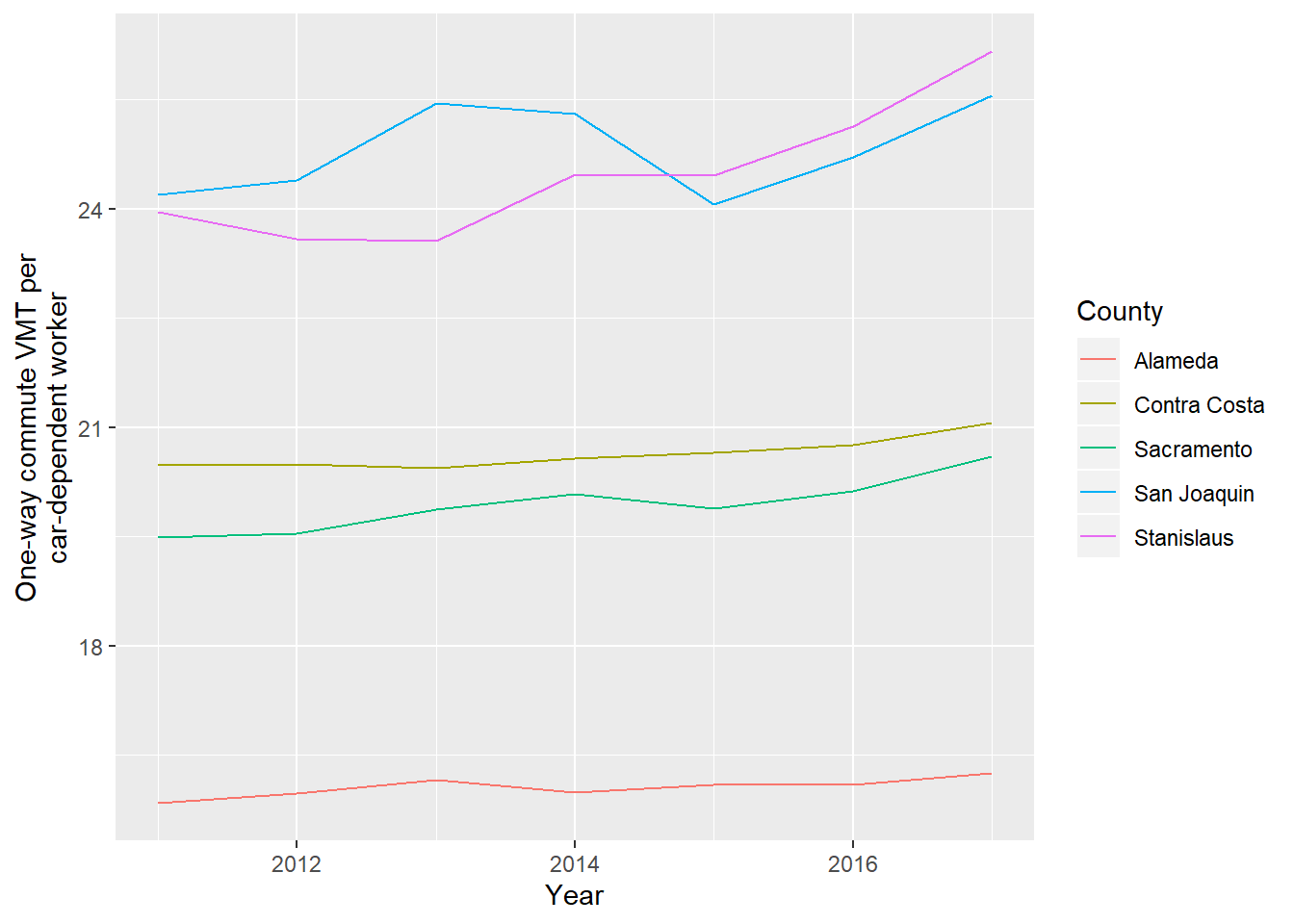
Figure 2.19: One-way commute miles per car-dependent worker by county, 2011 to 2017. Data from LODES.
\(~\)
One of the possible contributions to an increasing VMT/job isn’t necessarily further away jobs but less carpooling to get to those jobs. The following figure shows that the percent of car-dependent SJC workers who carpool has declined from 2015 to 2017, similar to Stanislaus and Sacramento County.
# county_modeshare <- NULL
#
# for(year in 2011:2017){
#   for(county in county_neighbors$COUNTYFP){
#
#     print(paste0(year,"-",county))
#
#     load(paste0("C:/Users/derek/Google Drive/City Systems/Stockton Green Economy/acs1_vars_",year,".Rdata"))
#
#     travel_time_mode <-
#     getCensus(
#       name = "acs/acs1",
#       vintage = year,
#       region = paste0("county:",county),
#       regionin = "state:06",
#       vars = "group(B08134)"
#     ) %>%
#     select_if(!names(.) %in% c("GEO_ID","state","NAME")) %>%
#     dplyr::select(-c(contains("EA"),contains("MA"),contains("M"))) %>%
#     gather(
#       key = "variable",
#       value = "estimate",
#       -county
#     ) %>%
#     mutate(
#       label = acs_vars$label[match(variable,acs_vars$name)],
#       time = # This extracts only the time information from our label.
#         substr(
#           label,
#           lapply(
#             label,
#             function(x){
#               ifelse(
#                 length(unlist(gregexpr('!!',x)))<3,
#                 NA,
#                 max(unlist(gregexpr('!!',x)))+2
#               )
#             }
#           ),
#           nchar(label)
#         ),
#       mode = # This extracts only the mode information from our label. It doesn't fully deal with double-counting, so some are further removed later on in a filter.
#         substr(
#           label,
#           lapply(
#             label,
#             function(x){
#               ifelse(
#                 length(unlist(gregexpr('!!',x)))<3,
#                 NA,
#                 unlist(gregexpr('!!',x))[length(unlist(gregexpr('!!',x)))-1]+2
#               )
#             }
#           ),
#           lapply(
#             label,
#             function(x){
#               max(unlist(gregexpr('!!',x)))-1
#             }
#           )
#         )
#     ) %>%
#     filter(!is.na(time)) %>% # This removes the grand total rows that are usually at the top of the ACS data.
#     filter(!mode %in% c("Car, truck, or van","Car truck or van","Carpooled","Public transportation (excluding taxicab)")) %>% # This removes double-counted subtotals.
#     dplyr::select(-variable,-label)
#
#     travel_time_mode_summary <-
#       travel_time_mode %>%
#       summarize(
#         jobs = sum(estimate),
#         jobs_drovealone = sum(estimate[which(mode == "Drove alone")]),
#         jobs_carpool2 = sum(estimate[which(mode == "In 2-person carpool")]),
#         jobs_carpool3 = sum(estimate[which(mode == "In 3-or-more-person carpool")]),
#       ) %>%
#       mutate(
#         vehicles_drovealone = jobs_drovealone,
#         vehicles_carpool2 = jobs_carpool2/2,
#         vehicles_carpool3 = jobs_carpool3/3,
#         jobs_car = jobs_drovealone+jobs_carpool2+jobs_carpool3,
#         jobs_carpool = jobs_carpool2+jobs_carpool3,
#         vehicles = vehicles_drovealone,vehicles_carpool2,vehicles_carpool3,
#         perc_jobs_car = jobs_car/jobs,
#         perc_jobs_carpool = jobs_carpool/jobs,
#         perc_vehicle = vehicles/jobs
#       )
#
#     county_modeshare <-
#       county_modeshare %>%
#       rbind(
#         data.frame(
#           year = year,
#           county = county,
#           jobs = travel_time_mode_summary$jobs,
#           perc_jobs_car = travel_time_mode_summary$perc_jobs_car,
#           perc_jobs_carpool = travel_time_mode_summary$perc_jobs_carpool,
#           perc_vehicle = travel_time_mode_summary$perc_vehicle
#         )
#       )
#   }
# }
#
# save(county_modeshare, file = "C:/Users/derek/Google Drive/City Systems/Stockton Green Economy/LODES/county_modeshare.Rdata")
# load("C:/Users/derek/Google Drive/City Systems/Stockton Green Economy/LODES/county_modeshare.Rdata")
#
# county_modeshare %>%
#   filter(county %in% c("077","001","013","067","099")) %>%
#   filter(jobs != 0) %>%
#   left_join(county_neighbors, by = c("county" = "COUNTYFP")) %>%
#   ggplot(
#     aes(
#       x = year,
#       y = perc_jobs_carpool/perc_jobs_car*100,
#       colour = NAME
#     )
#   ) +
#   geom_line() +
#   labs(x = "Year", y = "% Car-dependent workers who carpool") +
#   scale_color_discrete(name = "County")

county_commute_vmt_tractmode %>%
  left_join(county_neighbors, by = c("County" = "COUNTYFP")) %>%
  ggplot(
    aes(
      x = Year,
      y = jobs_carpool/jobs_car,
      colour = NAME
    )
  ) +
  geom_line() +
  labs(y = "% Car-dependent workers who carpool") +
  scale_color_discrete(name = "County")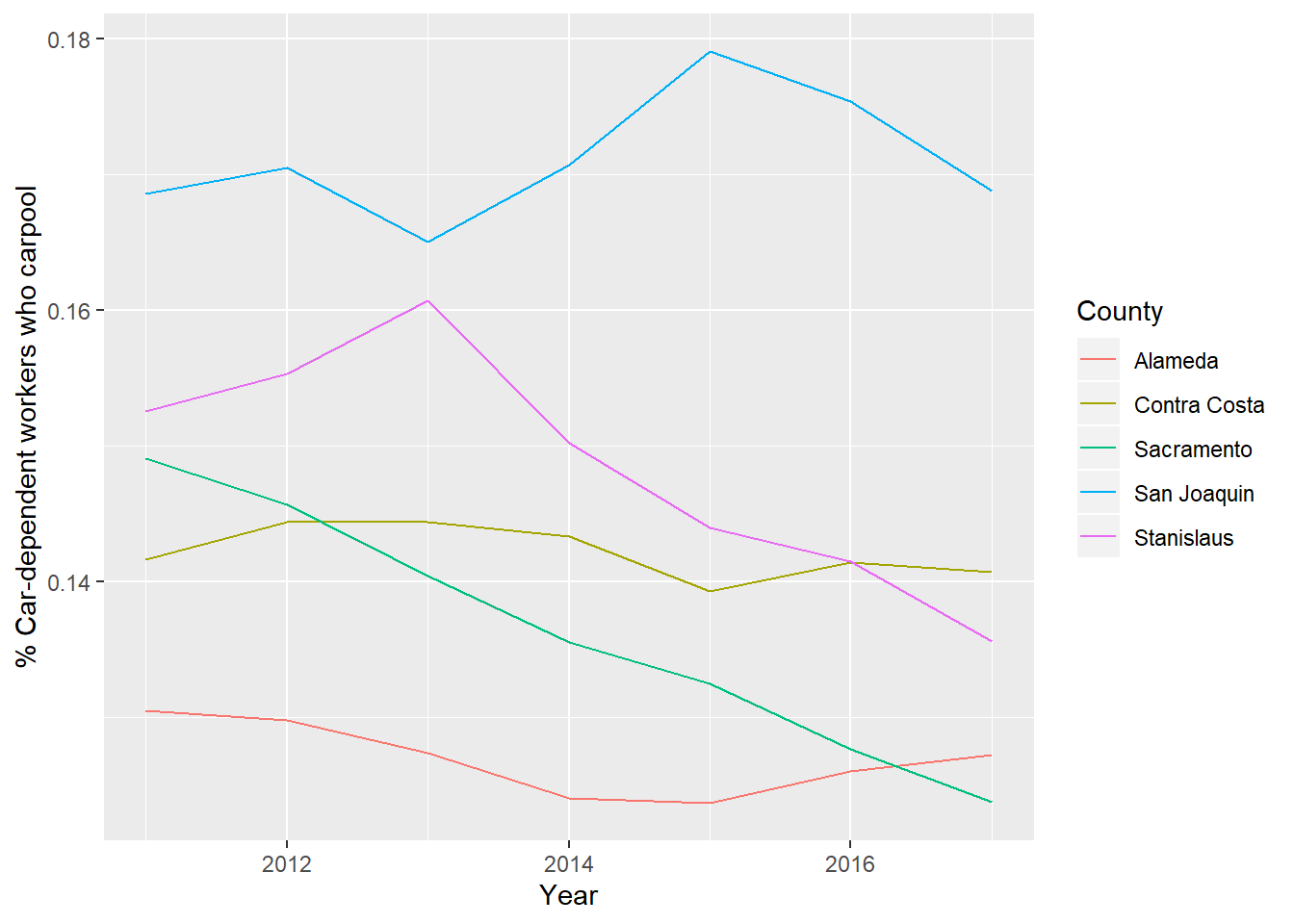
Figure 2.20: Percent of car-dependent commuters traveling by carpool, by county, 2011 to 2017. Data from LODES and ACS.
\(~\)
2.5.2 City-level Analysis
The following graph shows the distribution of workplaces by distance from home for Stockton residents.
# for(year in 2011:2017){
#
#   print(year)
#
#   ca_lodes <-
#     grab_lodes(
#       state = "ca",
#       year = year,
#       lodes_type = "od",
#       job_type = "JT01", #Primary Jobs
#       segment = "S000",
#       state_part = "main",
#       agg_geo = "bg"
#     )
#
#   stockton_lodes_h <-
#     ca_lodes[which(ca_lodes$h_bg %in% stockton_bgs_full$GEOID),]
#
#   stockton_lodes_h_origin_centroids <-
#     st_centroid(ca_bgs[which(ca_bgs$GEOID %in% stockton_lodes_h$h_bg),])
#
#   stockton_lodes_h_dest_centroids <-
#     st_centroid(ca_bgs[which(ca_bgs$GEOID %in% stockton_lodes_h$w_bg),])
#
#   route <-
#     1:nrow(stockton_lodes_h) %>%
#     map_dfr(function(row){
#       print(row)
#       route <- osrmRoute(
#         src = stockton_lodes_h_origin_centroids[which(stockton_lodes_h_origin_centroids$GEOID %in% stockton_lodes_h[row,"h_bg"]),],
#         dst = stockton_lodes_h_dest_centroids[which(stockton_lodes_h_dest_centroids$GEOID %in% stockton_lodes_h[row,"w_bg"]),],
#         overview = FALSE
#       ) %>%
#         as.list() %>%
#         as.data.frame()
#       if(is_empty(route)){
#         return(
#           data.frame(
#             duration = NA,
#             distance = NA
#           )
#         )
#       } else {return(route)}
#     })
#
#   stockton_lodes_h_route <-
#     stockton_lodes_h %>%
#     cbind(route)
#
#   stockton_lodes_h_filter <-
#     stockton_lodes_h_route %>%
#     filter(duration < 180)
#
#   save(stockton_lodes_h_route,stockton_lodes_h_filter, file = paste0("C:/Users/derek/Google Drive/City Systems/Stockton Green Economy/LODES/stockton_lodes_",year,".Rdata"))
# }

load("C:/Users/derek/Google Drive/City Systems/Stockton Green Economy/LODES/stockton_lodes_2017_tract.Rdata")

ggplot(
  stockton_lodes_h_filter,
  aes(
    x = as.numeric(distance)/1.60934,
    weight = S000
  )
) +
  geom_histogram(binwidth = 5) +
  labs(title = "Workplace Commute Distance to Work for Stockton Employed Residents", x = "Commute Distance to Work, Miles", y = "Number of Residents")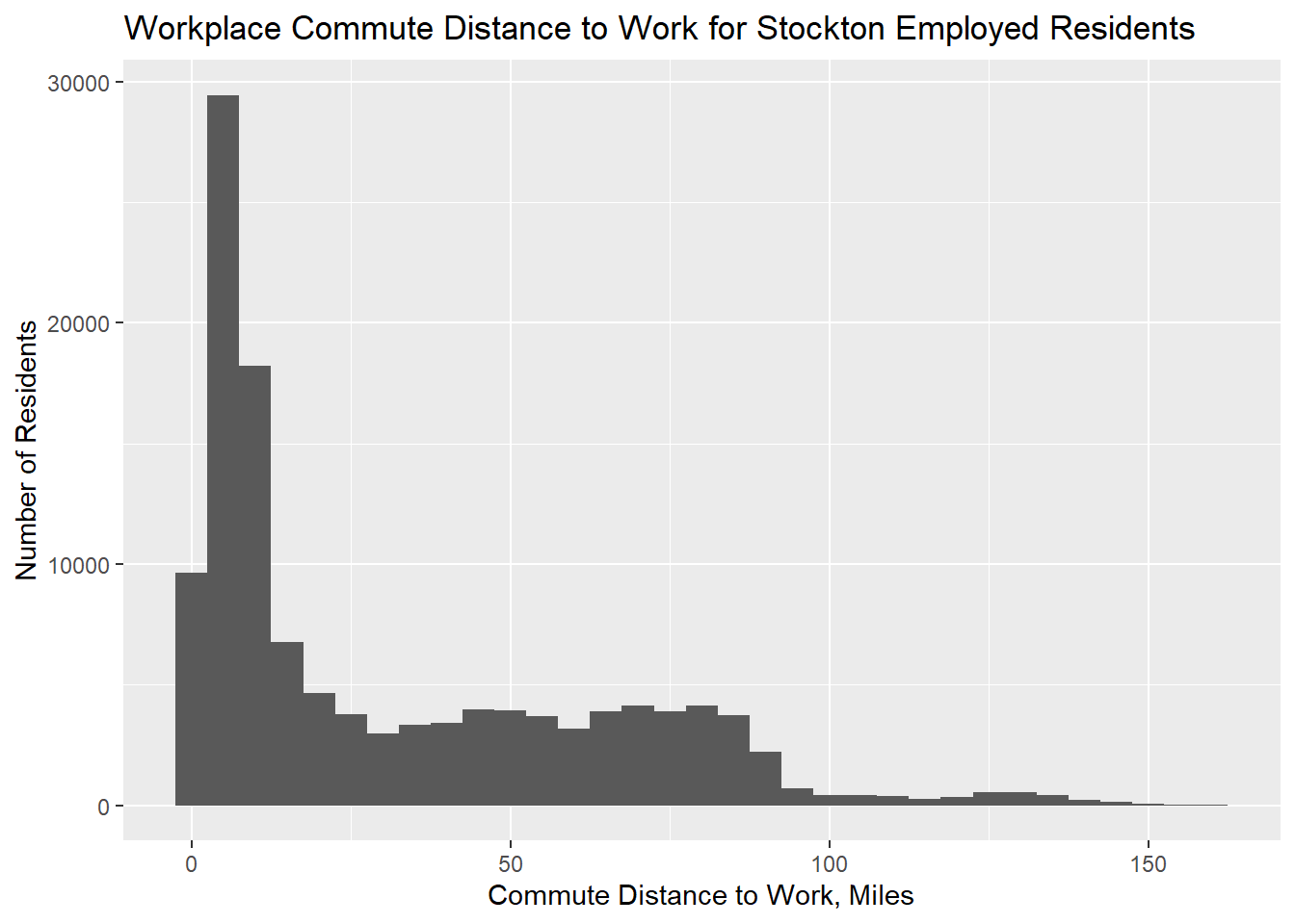
Figure 2.21: Distribution of workplaces by distance from home for Stockton employed residents. Trips greater than 3 hours are removed. Data from LODES, 2017.
\(~\)
The map below demonstrates the extent of geographic spread of Stockton residents across the greater Northern California region, potentially on a day-to-day basis. Most of the tracts shown have only a handful of estimated Stockton workers, but interesting concentrations of workers can be seen by zooming in and hovering over areas like the East Bay.
stockton_jobs_map <-
  stockton_lodes_h_filter %>%
  group_by(w_tract) %>%
  summarize(
    `Jobs held by Stockton residents` = sum(S000, na.rm=T)
  ) %>%
  left_join(ca_tracts, by = c("w_tract" = "GEOID")) %>%
  st_as_sf()

# map = mapview(stockton_jobs_map[,c("Jobs held by Stockton residents")], zcol = "Jobs held by Stockton residents", col.regions = colorRampPalette(c("snow", "black", "grey")), map.types = c("OpenStreetMap"), legend = TRUE, layer.name = 'Jobs held by</br>Stockton residents')
#
# mapshot(map,url="map-stockton-jobs-map.html")

knitr::include_url("https://citysystems.github.io/stockton-greeneconomy/map-stockton-jobs-map.html")
Figure 2.22: Tracts where Stockton residents work - number of jobs. Data from LODES, 2017.
\(~\)
The previous map can be considered in combination with the map below, which essentially shows the average distance in miles traveled one-way by Stockton workers to those tracts. Evidently, workers traveling to further-away tracts are responsible for a disproportionate share of the transportation emissions compared to other Stockton workers.
stockton_commute_avg <-
  stockton_lodes_h_filter %>%
  group_by(w_tract) %>%
  summarize(
    `Average Commute Time, Hours` = mean(duration, na.rm=T)
  ) %>%
  left_join(ca_tracts, by = c("w_tract" = "GEOID")) %>%
  st_as_sf()

# map = mapview(stockton_commute_avg[,c("Average Commute Time, Hours")], zcol = "Average Commute Time, Hours", map.types = c("OpenStreetMap"), legend = TRUE, layer.name = 'Average Commute</br>Time, Hours')
#
# mapshot(map,url="map-stockton-commute-avg.html")

knitr::include_url("https://citysystems.github.io/stockton-greeneconomy/map-stockton-commute-avg.html")
Figure 2.23: Tracts where Stockton residents work - average commute time, in hours. Data from LODES, 2017.
\(~\)
Similar to the county-level analysis, we calculated the change in VMT/job over time, which might give more important relative insight given the many assumptions that go into the specific quantity of VMTs in any given year.
load("C:/Users/derek/Google Drive/City Systems/Stockton Green Economy/LODES/stockton_commute_vmt_tractmode.Rdata")

stockton_commute_vmt_tractmode_table <-
  stockton_commute_vmt_tractmode %>%
  transmute(
    Year = Year,
    `Commute One-Way VMT` = prettyNum(round(vmt,-3), big.mark=","),
    `Workers` = prettyNum(round(jobs,-3), big.mark=","),
    `One-Way VMT/Workers` = round(vmt/jobs_car,1),
    `% Car-Dependent Workers who Carpool` = paste0(round(jobs_carpool/jobs_car*100,1),"%")
  )

kable(
  stockton_commute_vmt_tractmode_table,
  booktabs = TRUE,
  caption = 'Stockton commute one-way VMT from 2011-2017. Data from LODES and ACS 1-yr.'
) %>%
  kable_styling() %>%
scroll_box(width = "100%")| Year | Commute One-Way VMT | Workers | One-Way VMT/Workers | % Car-Dependent Workers who Carpool |
|---|---|---|---|---|
| 2011 | 1,837,000 | 98,000 | 20.3 | 18.2% |
| 2012 | 1,932,000 | 99,000 | 20.9 | 18.3% |
| 2013 | 1,979,000 | 102,000 | 20.9 | 19% |
| 2014 | 2,228,000 | 108,000 | 22.0 | 20.1% |
| 2015 | 2,226,000 | 114,000 | 21.0 | 20.2% |
| 2016 | 2,389,000 | 119,000 | 21.5 | 19.8% |
| 2017 | 2,635,000 | 123,000 | 23.0 | 18.8% |
\(~\)
The average one-way commute trip for the Stockton worker appears to have increased by 13% over the last 6 years. This could be explained by existing residents changing to jobs that are further and further away from home, where better employment opportunities can be found, and by new residents moving to Stockton to find affordable housing but retaining their faraway jobs.
The following figure compares Stockton and SJC VMT/job. The trends are similar, though Stockton residents commute less distance than SJC residents overall.
# stockton_commute_vmt_bgmode <- NULL
#
# for(year in 2011:2017){
#     print(year)
#
#     load(paste0("C:/Users/derek/Google Drive/City Systems/Stockton Green Economy/LODES/stockton_lodes_",year,".Rdata"))
#
#     load(paste0("C:/Users/derek/Google Drive/City Systems/Stockton Green Economy/acs5_vars_",year,".Rdata"))
#
#     travel_time_mode <-
#       getCensus(
#         name = "acs/acs5",
#         vintage = ifelse(
#           year < 2013,
#           2013,
#           year
#         ),
#         region = "block group:*",
#         regionin = "state:06+county:077",
#         vars = "group(B08134)"
#       ) %>%
#       mutate(bg = paste0(state,county,tract,block_group)) %>%
#       select_if(!names(.) %in% c("GEO_ID","state","county","tract","block_group","NAME")) %>%
#       dplyr::select(-c(contains("EA"),contains("MA"),contains("M"))) %>%
#       gather(
#         key = "variable",
#         value = "estimate",
#         -bg
#       ) %>%
#       mutate(
#         label = acs_vars$label[match(variable,acs_vars$name)],
#         time = # This extracts only the time information from our label.
#           substr(
#             label,
#             lapply(
#               label,
#               function(x){
#                 ifelse(
#                   length(unlist(gregexpr('!!',x)))<3,
#                   NA,
#                   max(unlist(gregexpr('!!',x)))+2
#                 )
#               }
#             ),
#             nchar(label)
#           ),
#         mode = # This extracts only the mode information from our label. It doesn't fully deal with double-counting, so some are further removed later on in a filter.
#           substr(
#             label,
#             lapply(
#               label,
#               function(x){
#                 ifelse(
#                   length(unlist(gregexpr('!!',x)))<3,
#                   NA,
#                   unlist(gregexpr('!!',x))[length(unlist(gregexpr('!!',x)))-1]+2
#                 )
#               }
#             ),
#             lapply(
#               label,
#               function(x){
#                 max(unlist(gregexpr('!!',x)))-1
#               }
#             )
#           )
#       ) %>%
#       filter(!is.na(time)) %>% # This removes the grand total rows that are usually at the top of the ACS data.
#       filter(!mode %in% c("Car, truck, or van","Car truck or van","Carpooled","Public transportation (excluding taxicab)")) %>% # This removes double-counted subtotals.
#       dplyr::select(-variable,-label)
#
#     travel_time_mode_summary <-
#       travel_time_mode %>%
#       group_by(bg,time) %>%
#       summarize(
#         jobs = sum(estimate),
#         jobs_drovealone = sum(estimate[which(mode == "Drove alone")]),
#         jobs_carpool2 = sum(estimate[which(mode == "In 2-person carpool")]),
#         jobs_carpool3 = sum(estimate[which(mode == "In 3-or-more-person carpool")]),
#       ) %>%
#       mutate(
#         vehicles_drovealone = jobs_drovealone,
#         vehicles_carpool2 = jobs_carpool2/2,
#         vehicles_carpool3 = jobs_carpool3/3,
#         jobs_car = jobs_drovealone+jobs_carpool2+jobs_carpool3,
#         jobs_carpool = jobs_carpool2+jobs_carpool3,
#         vehicles = vehicles_drovealone,vehicles_carpool2,vehicles_carpool3,
#         perc_jobs_car = jobs_car/jobs,
#         perc_jobs_carpool = jobs_carpool/jobs,
#         perc_vehicle = vehicles/jobs
#       )
#
#   stockton_lodes_h_mode <-
#     stockton_lodes_h_filter %>%
#     transmute(
#       residence = h_bg,
#       jobs = S000,
#       duration = duration,
#       person_miles = S000*as.numeric(distance)/1.60934,
#       person_hours = S000*as.numeric(duration)/60
#     ) %>%
#     mutate(
#       tier =
#         case_when(
#           duration < 10 ~ "Less than 10 minutes",
#           duration < 15 ~ "10 to 14 minutes",
#           duration < 20 ~ "15 to 19 minutes",
#           duration < 25 ~ "20 to 24 minutes",
#           duration < 30 ~ "25 to 29 minutes",
#           duration < 35 ~ "30 to 34 minutes",
#           duration < 45 ~ "35 to 44 minutes",
#           duration < 60 ~ "45 to 59 minutes",
#           TRUE ~ "60 or more minutes"
#         )
#     ) %>%
#     left_join(
#       travel_time_mode_summary %>%
#         dplyr::select(
#           bg,
#           time,
#           perc_jobs_car,
#           perc_jobs_carpool,
#           perc_vehicle
#         ),
#       by = c("residence" = "bg", "tier" = "time")
#     ) %>%
#     mutate(
#       jobs_car = jobs*perc_jobs_car,
#       jobs_carpool = jobs*perc_jobs_carpool,
#       vehicles = jobs*perc_vehicle,
#       vmt = person_miles*perc_vehicle
#     )
#
#     stockton_commute_vmt_bgmode <-
#       rbind(stockton_commute_vmt_bgmode,
#         data.frame(
#           Year = year,
#           person_miles = sum(stockton_lodes_h_mode$person_miles, na.rm=T),
#           jobs = sum(stockton_lodes_h_mode$jobs, na.rm=T),
#           jobs_car = sum(stockton_lodes_h_mode$jobs_car, na.rm=T),
#           jobs_carpool = sum(stockton_lodes_h_mode$jobs_carpool, na.rm=T),
#           vehicles = sum(stockton_lodes_h_mode$vehicles, na.rm = T),
#           vmt = sum(stockton_lodes_h_mode$vmt, na.rm=T)
#         )
#       )
#
#     save(stockton_commute_vmt_bgmode,file = "C:/Users/derek/Google Drive/City Systems/Stockton Green Economy/LODES/stockton_commute_vmt_bgmode.Rdata")
# }
#
# stockton_commute_vmt_tractmode <- NULL
#
# for(year in 2011:2017){
#     print(year)
#
#     load(paste0("C:/Users/derek/Google Drive/City Systems/Stockton Green Economy/LODES/stockton_lodes_",year,"_tract.Rdata"))
#
#     load(paste0("C:/Users/derek/Google Drive/City Systems/Stockton Green Economy/acs5_vars_",year,".Rdata"))
#
#     travel_time_mode <-
#       getCensus(
#         name = "acs/acs5",
#         vintage = year,
#         region = "tract:*",
#         regionin = "state:06+county:077",
#         vars = "group(B08134)"
#       ) %>%
#       mutate(tract = paste0(state,county,tract)) %>%
#       select_if(!names(.) %in% c("GEO_ID","state","county","NAME")) %>%
#       dplyr::select(-c(contains("EA"),contains("MA"),contains("M"))) %>%
#       gather(
#         key = "variable",
#         value = "estimate",
#         -tract
#       ) %>%
#       mutate(
#         label = acs_vars$label[match(variable,acs_vars$name)],
#         time = # This extracts only the time information from our label.
#           substr(
#             label,
#             lapply(
#               label,
#               function(x){
#                 ifelse(
#                   length(unlist(gregexpr('!!',x)))<3,
#                   NA,
#                   max(unlist(gregexpr('!!',x)))+2
#                 )
#               }
#             ),
#             nchar(label)
#           ),
#         mode = # This extracts only the mode information from our label. It doesn't fully deal with double-counting, so some are further removed later on in a filter.
#           substr(
#             label,
#             lapply(
#               label,
#               function(x){
#                 ifelse(
#                   length(unlist(gregexpr('!!',x)))<3,
#                   NA,
#                   unlist(gregexpr('!!',x))[length(unlist(gregexpr('!!',x)))-1]+2
#                 )
#               }
#             ),
#             lapply(
#               label,
#               function(x){
#                 max(unlist(gregexpr('!!',x)))-1
#               }
#             )
#           )
#       ) %>%
#       filter(!is.na(time)) %>% # This removes the grand total rows that are usually at the top of the ACS data.
#       filter(!mode %in% c("Car, truck, or van","Car truck or van","Carpooled","Public transportation (excluding taxicab)")) %>% # This removes double-counted subtotals.
#       dplyr::select(-variable,-label)
#
#     travel_time_mode_summary <-
#       travel_time_mode %>%
#       group_by(tract,time) %>%
#       summarize(
#         jobs = sum(estimate),
#         jobs_drovealone = sum(estimate[which(mode == "Drove alone")]),
#         jobs_carpool2 = sum(estimate[which(mode == "In 2-person carpool")]),
#         jobs_carpool3 = sum(estimate[which(mode == "In 3-or-more-person carpool")]),
#       ) %>%
#       mutate(
#         vehicles_drovealone = jobs_drovealone,
#         vehicles_carpool2 = jobs_carpool2/2,
#         vehicles_carpool3 = jobs_carpool3/3,
#         jobs_car = jobs_drovealone+jobs_carpool2+jobs_carpool3,
#         jobs_carpool = jobs_carpool2+jobs_carpool3,
#         vehicles = vehicles_drovealone,vehicles_carpool2,vehicles_carpool3,
#         perc_jobs_car = jobs_car/jobs,
#         perc_jobs_carpool = jobs_carpool/jobs,
#         perc_vehicle = vehicles/jobs
#       )
#
#   stockton_lodes_h_mode <-
#     stockton_lodes_h_filter %>%
#     transmute(
#       residence = h_tract,
#       jobs = S000,
#       duration = duration,
#       person_miles = S000*as.numeric(distance)/1.60934,
#       person_hours = S000*as.numeric(duration)/60
#     ) %>%
#     mutate(
#       tier =
#         case_when(
#           duration < 10 ~ "Less than 10 minutes",
#           duration < 15 ~ "10 to 14 minutes",
#           duration < 20 ~ "15 to 19 minutes",
#           duration < 25 ~ "20 to 24 minutes",
#           duration < 30 ~ "25 to 29 minutes",
#           duration < 35 ~ "30 to 34 minutes",
#           duration < 45 ~ "35 to 44 minutes",
#           duration < 60 ~ "45 to 59 minutes",
#           TRUE ~ "60 or more minutes"
#         )
#     ) %>%
#     left_join(
#       travel_time_mode_summary %>%
#         dplyr::select(
#           tract,
#           time,
#           perc_jobs_car,
#           perc_jobs_carpool,
#           perc_vehicle
#         ),
#       by = c("residence" = "tract", "tier" = "time")
#     ) %>%
#     mutate(
#       jobs_car = jobs*perc_jobs_car,
#       jobs_carpool = jobs*perc_jobs_carpool,
#       vehicles = jobs*perc_vehicle,
#       vmt = person_miles*perc_vehicle
#     )
#
#     stockton_commute_vmt_tractmode <-
#       rbind(stockton_commute_vmt_tractmode,
#         data.frame(
#           Year = year,
#           person_miles = sum(stockton_lodes_h_mode$person_miles, na.rm=T),
#           jobs = sum(stockton_lodes_h_mode$jobs, na.rm=T),
#           jobs_car = sum(stockton_lodes_h_mode$jobs_car, na.rm=T),
#           jobs_carpool = sum(stockton_lodes_h_mode$jobs_carpool, na.rm=T),
#           vehicles = sum(stockton_lodes_h_mode$vehicles, na.rm = T),
#           vmt = sum(stockton_lodes_h_mode$vmt, na.rm=T)
#         )
#       )
#
#     save(stockton_commute_vmt_tractmode,file = "C:/Users/derek/Google Drive/City Systems/Stockton Green Economy/LODES/stockton_commute_vmt_tractmode.Rdata")
# }
# load("C:/Users/derek/Google Drive/City Systems/Stockton Green Economy/LODES/stockton_commute_vmt_tractmode.Rdata")
#
# stockton_commute_vmt_tractmode %>%
#   ggplot(
#     aes(
#       x = Year,
#       y = vmt/jobs
#     )
#   ) +
#   geom_line()
#
# stockton_commute_vmt_countymode <- NULL
#
# for(year in 2011:2017){
#
#   print(year)
#
#   load(paste0("C:/Users/derek/Google Drive/City Systems/Stockton Green Economy/LODES/stockton_lodes_",year,"_tract.Rdata"))
#
#   load(paste0("C:/Users/derek/Google Drive/City Systems/Stockton Green Economy/acs1_vars_",year,".Rdata"))
#
#   travel_time_mode <-
#     getCensus(
#       name = "acs/acs1",
#       vintage = year,
#       region = "county:077",
#       regionin = "state:06",
#       vars = "group(B08134)"
#     ) %>%
#     select_if(!names(.) %in% c("GEO_ID","state","NAME")) %>%
#     dplyr::select(-c(contains("EA"),contains("MA"),contains("M"))) %>%
#     gather(
#       key = "variable",
#       value = "estimate",
#       -county
#     ) %>%
#     mutate(
#       label = acs_vars$label[match(variable,acs_vars$name)],
#       time = # This extracts only the time information from our label.
#         substr(
#           label,
#           lapply(
#             label,
#             function(x){
#               ifelse(
#                 length(unlist(gregexpr('!!',x)))<3,
#                 NA,
#                 max(unlist(gregexpr('!!',x)))+2
#               )
#             }
#           ),
#           nchar(label)
#         ),
#       mode = # This extracts only the mode information from our label. It doesn't fully deal with double-counting, so some are further removed later on in a filter.
#         substr(
#           label,
#           lapply(
#             label,
#             function(x){
#               ifelse(
#                 length(unlist(gregexpr('!!',x)))<3,
#                 NA,
#                 unlist(gregexpr('!!',x))[length(unlist(gregexpr('!!',x)))-1]+2
#               )
#             }
#           ),
#           lapply(
#             label,
#             function(x){
#               max(unlist(gregexpr('!!',x)))-1
#             }
#           )
#         )
#     ) %>%
#     filter(!is.na(time)) %>% # This removes the grand total rows that are usually at the top of the ACS data.
#     filter(!mode %in% c("Car, truck, or van","Car truck or van","Carpooled","Public transportation (excluding taxicab)")) %>% # This removes double-counted subtotals.
#     dplyr::select(-variable,-label)
#
#     travel_time_mode_summary <-
#       travel_time_mode %>%
#       group_by(time) %>%
#       summarize(
#         jobs = sum(estimate),
#         jobs_drovealone = sum(estimate[which(mode == "Drove alone")]),
#         jobs_carpool2 = sum(estimate[which(mode == "In 2-person carpool")]),
#         jobs_carpool3 = sum(estimate[which(mode == "In 3-or-more-person carpool")]),
#       ) %>%
#       mutate(
#         vehicles_drovealone = jobs_drovealone,
#         vehicles_carpool2 = jobs_carpool2/2,
#         vehicles_carpool3 = jobs_carpool3/3,
#         jobs_car = jobs_drovealone+jobs_carpool2+jobs_carpool3,
#         jobs_carpool = jobs_carpool2+jobs_carpool3,
#         vehicles = vehicles_drovealone,vehicles_carpool2,vehicles_carpool3,
#         perc_jobs_car = jobs_car/jobs,
#         perc_jobs_carpool = jobs_carpool/jobs,
#         perc_vehicle = vehicles/jobs
#       )
#
#   stockton_lodes_h_mode <-
#     stockton_lodes_h_filter %>%
#     transmute(
#       jobs = S000,
#       duration = duration,
#       person_miles = S000*as.numeric(distance)/1.60934,
#       person_hours = S000*as.numeric(duration)/60
#     ) %>%
#     mutate(
#       tier =
#         case_when(
#           duration < 10 ~ "Less than 10 minutes",
#           duration < 15 ~ "10 to 14 minutes",
#           duration < 20 ~ "15 to 19 minutes",
#           duration < 25 ~ "20 to 24 minutes",
#           duration < 30 ~ "25 to 29 minutes",
#           duration < 35 ~ "30 to 34 minutes",
#           duration < 45 ~ "35 to 44 minutes",
#           duration < 60 ~ "45 to 59 minutes",
#           TRUE ~ "60 or more minutes"
#         )
#     ) %>%
#     left_join(
#       travel_time_mode_summary %>%
#         dplyr::select(
#           time,
#           perc_jobs_car,
#           perc_jobs_carpool,
#           perc_vehicle
#         ),
#       by = c("tier" = "time")
#     ) %>%
#     mutate(
#       jobs_car = jobs*perc_jobs_car,
#       jobs_carpool = jobs*perc_jobs_carpool,
#       vehicles = jobs*perc_vehicle,
#       vmt = person_miles*perc_vehicle
#     )
#
#     stockton_commute_vmt_countymode <-
#       rbind(stockton_commute_vmt_countymode,
#         data.frame(
#           Year = year,
#           person_miles = sum(stockton_lodes_h_mode$person_miles, na.rm=T),
#           jobs = sum(stockton_lodes_h_mode$jobs, na.rm=T),
#           jobs_car = sum(stockton_lodes_h_mode$jobs_car, na.rm=T),
#           jobs_carpool = sum(stockton_lodes_h_mode$jobs_carpool, na.rm=T),
#           vehicles = sum(stockton_lodes_h_mode$vehicles, na.rm = T),
#           vmt = sum(stockton_lodes_h_mode$vmt, na.rm=T)
#         )
#       )
# }
#
# save(stockton_commute_vmt_countymode, file = "C:/Users/derek/Google Drive/City Systems/Stockton Green Economy/LODES/stockton_commute_vmt_countymode.Rdata")
# load("C:/Users/derek/Google Drive/City Systems/Stockton Green Economy/LODES/stockton_commute_vmt_countymode.Rdata")
#
# stockton_commute_vmt_countymode %>%
#   ggplot(
#     aes(
#       x = Year,
#       y = vmt/jobs
#     )
#   ) +
#   geom_line()
#
# load("C:/Users/derek/Google Drive/City Systems/Stockton Green Economy/LODES/stockton_commute_vmt_bgmode.Rdata")
#
# load("C:/Users/derek/Google Drive/City Systems/Stockton Green Economy/LODES/stockton_commute_vmt_tractmode.Rdata")
#
# load("C:/Users/derek/Google Drive/City Systems/Stockton Green Economy/LODES/stockton_commute_vmt_countymode.Rdata")
#
# stockton_commute_vmt_compare <-
#   rbind(
#     stockton_commute_vmt_bgmode %>%
#       mutate(mode = "block group"),
#     stockton_commute_vmt_tractmode %>%
#       mutate(mode = "tract"),
#     stockton_commute_vmt_countymode %>%
#       mutate(mode = "county")
#   )
#
# stockton_commute_vmt_compare %>%
#   ggplot(
#     aes(
#       x = Year,
#       y = vmt/jobs,
#       linetype = mode
#     )
#   ) +
#   geom_line()

county_commute_vmt_tractmode %>%
  filter(County == "077") %>%
  ggplot(
    aes(
      x = Year,
      y = vmt/jobs_car,
      linetype = "SJC"
    )
  ) +
  geom_line() +
  geom_line(
    data = stockton_commute_vmt_tractmode,
    aes(
      x = Year,
      y = vmt/jobs_car,
      linetype = "Stockton"
    )
  ) +
  labs(y = "One-way commute miles\nper car-dependent worker", linetype = "Group")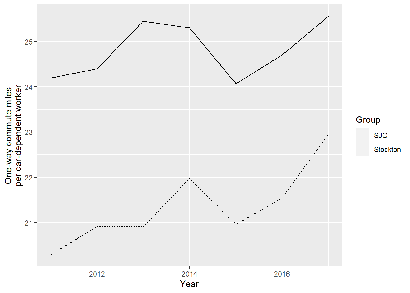
Figure 2.24: One-way commute miles per car-dependent worker in Stockton vs. SJC, 2011 to 2017. Data from LODES.
\(~\)
The following figure compares the percent of car-dependent workers who carpool in Stockton and SJC. Stockton workers overall are more likely to carpool than SJC workers overall, but the trends are again similar between Stockton and SJC, with a decline in carpooling in the last two years of data.
load("C:/Users/derek/Google Drive/City Systems/Stockton Green Economy/LODES/stockton_commute_vmt_tractmode.Rdata")

load("C:/Users/derek/Google Drive/City Systems/Stockton Green Economy/LODES/county_commute_vmt_tractmode.Rdata")

stockton_county_commute_vmt_compare <-
  rbind(
    county_commute_vmt_tractmode %>%
      filter(County == "077") %>%
      dplyr::select(-County) %>%
      mutate(type = "SJC"),
    stockton_commute_vmt_tractmode %>%
      mutate(type = "Stockton")
  )

stockton_county_commute_vmt_compare %>%
  ggplot(
    aes(
      x = Year,
      y = jobs_carpool/jobs_car*100,
      linetype = type
    )
  ) +
  geom_line() +
  labs(y = "% Car-dependent workers who carpool", linetype = "Group")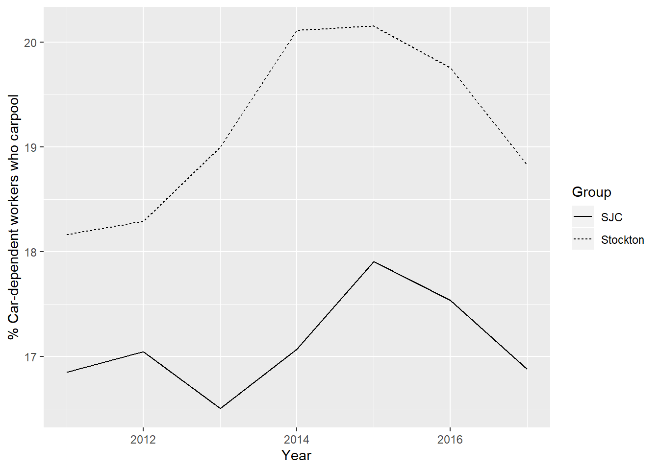
Figure 2.25: Percent of car-dependent commuters traveling by carpool, Stockton vs. SJC, 2011 to 2017. Data from LODES and ACS.
\(~\)