2.3 2005-2016 GHG Inventory
The State of California Governor’s Office of Planning and Research recommends that California local governments follow ICLEI’s Community Greenhouse Gas Emissions Protocol when undertaking their greenhouse gas emissions inventories. ICLEI helped to produce Stockton’s most recent GHG Inventory in 2016 which was compared to the previous inventory produced by ICF for the 2005 baseline year. The results from that report are copied below.
iclei_2005_2016 <-
  data.frame(
    "Year" = c(2005,2016),
    "Transportation" = c(1308696,1344846.19),
    "Solid Waste" = c(65720,61175),
    "Water/Wastewater" = c(115511,321486.42),
    "Agriculture" = c(928,947.298),
    "Commercial Energy" = c(369354,192191),
    "Industrial Energy" = c(60802,746225.84),
    "Residential Energy" = c(345862,267466),
    "Fugitive Emissions" = c(113080,159578.1397)
  ) %>%
  rename(
    `Solid Waste` = Solid.Waste,
    `Water/Wastewater` = Water.Wastewater,
    `Commercial Energy` = Commercial.Energy,
    `Industrial Energy` = Industrial.Energy,
    `Residential Energy` = Residential.Energy,
    `Fugitive Emissions` = Fugitive.Emissions
  )

iclei_2005_2016_plot <-
  iclei_2005_2016 %>%
  gather(
    key = "Type",
    value = "tCO2e",
    -Year
  ) %>%
  arrange(Year,desc(tCO2e))

iclei_2005_2016_table <-
  iclei_2005_2016 %>%
  transmute(
    Year = Year,
    Transportation = prettyNum(round(Transportation,-3),big.mark = ","),
    `Solid Waste` = prettyNum(round(`Solid Waste`,-3),big.mark = ","),
    `Water/Wastewater` = prettyNum(round(`Water/Wastewater`,-3),big.mark = ","),
    Agriculture = prettyNum(round(Agriculture,-2),big.mark = ","),
    `Commercial Energy` = prettyNum(round(`Commercial Energy`,-3),big.mark = ","),
    `Industrial Energy` = prettyNum(round(`Industrial Energy`,-3),big.mark = ","),
    `Residential Energy` = prettyNum(round(`Residential Energy`,-3),big.mark = ","),
    `Fugitive Emissions` = prettyNum(round(`Fugitive Emissions`,-3),big.mark = ",")
  )

kable(
  iclei_2005_2016_table,
  booktabs = TRUE,
  caption = 'Inventory comparisons for Stockton 2005-2016, from ICLEI. All units are in tCO2e.'
  ) %>%
  kable_styling() %>%
scroll_box(width = "100%")| Year | Transportation | Solid Waste | Water/Wastewater | Agriculture | Commercial Energy | Industrial Energy | Residential Energy | Fugitive Emissions |
|---|---|---|---|---|---|---|---|---|
| 2005 | 1,309,000 | 66,000 | 116,000 | 900 | 369,000 | 61,000 | 346,000 | 113,000 |
| 2016 | 1,345,000 | 61,000 | 321,000 | 900 | 192,000 | 746,000 | 267,000 | 160,000 |
\(~\)
iclei_2005_2016_plot %>%
  mutate(
    Year = factor(
      as.character(Year),
      levels =
        c(
          "2016",
          "2005"
        )
      ),
    Type = factor(
      Type,
      levels =
        c(
          "Transportation",
          "Solid Waste",
          "Water/Wastewater",
          "Agriculture",
          "Commercial Energy",
          "Industrial Energy",
          "Residential Energy",
          "Fugitive Emissions"
        )
    )
  ) %>%
  ggplot() +
  geom_bar(
    aes(
      fill = Type,
      x = Year,
      weight = `tCO2e`
    ),
    position = "stack"
  ) +
  coord_flip() +
  theme(legend.position = "bottom") +
  labs(title = "GHG Inventory Comparisons for Stockton, 2005-2016", x = "Year", y = "tCO2e")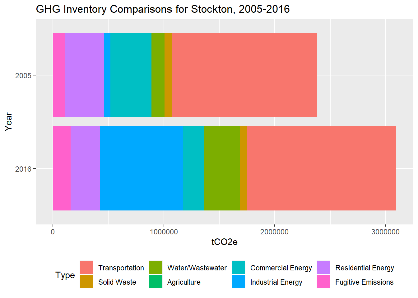
Figure 2.9: Inventory comparisons for Stockton 2005-2016, from ICLEI.
\(~\)
It is not within the scope of this project to formally update the 2016 ICLEI GHG Inventory for 2018, which is best completed by ICLEI or another similar organization. In fact, many of the significant components of ICLEI’s formal GHG analysis, like “Water Energy” for example, are simply based off of an interpolation of population changes, given the lack of official data – in other words, it is similar to what we have already done to project GHGs to 2040. We believe the following three focus areas are essential:
- Normalization of the emissions by the incremental unit of activity, which is usually population, to understand the baseline rate of GHG emissions per actor. Unless we intend to directly limit the number of actors, these activity emission rates are fundamentally the factors that determine how large Stockton’s footprint is. The reduction of activity emissions rates therefore becomes the critical problem to solve, either through behavior change, technology, or other means. We have already normalized overall emission sectors by jobs and population, but to get to the level of concrete green economy strategies, we will need to disaggregate further by specific key activities. The next few sections pursue this goal, focusing on some of the largest emitting activities: passenger vehicle driving and building energy.
- Focusing on activity emissions rates also requires having direct measurement data in those same activity sectors to be able to calibrate our rates. For the two sectors we will focus on in the subsequent sections, passenger vehicle driving and building energy, there are fortunately recent public data sources we can use to calibrate our baseline rates, and we can expect these data sources to be available in the future so we can check whether rates have fallen in the ways we will have been hoping for, given our various strategic interventions. Part of our contribution through this project is to prepare scripts that can more easily update measurements in the future as soon as new public data is available, so that feedback can be obtained as efficiently as possible. These scripts also essentially help to update the most significant components of an overall GHG inventory analysis.
- Since the availability of direct measurement data is critical to both the updating of GHG inventories and the understanding of the efficacy of our investments, we should also seek to increase the availability of direct measurement data in the sectors in which it is less readily available. These areas include industrial energy consumption (which is often restricted because of the California Public Utilities Commission’s 15/15 rule, which means that utilities cannot provide data at aggregations with fewer than 15 customers or one customer greater than 15% of usage), water consumption (given the existence of private water providers), and waste production specific to Stockton residents (given that data is collected at the landfill but isn’t disaggregated by truck routes or individual properties). These are all areas with opportunity for novel data sharing agreements to be negotiated by the City (e.g. the PG&E Green Communities Program, which effectively will enlist PG&E to directly complete the 3 steps outlined here for Stockton’s building energy sector), and these efforts will improve the overall green economy initiative.
The following table shows a preliminary normalization of the 2005 and 2016 GHG emissions by residents and jobs, using the following allocation:
- Residential Energy and Transportation were allocated entirely to residents
- Commercial Energy, Agriculture, and Fugitive Emissions were allocated entirely to jobs
- Solid Waste and Water/Wastewater were distributed proportionally between residents and jobs
- Industrial Energy was not included, given the significant difference in methodology between 2005 and 2016 as documented by ICLEI
# ca_wac_2005 <-
#   grab_lodes(
#     state = "ca",
#     year = 2005,
#     lodes_type = "wac",
#     job_type = "JT01",
#     segment = "S000",
#     state_part = "main",
#     agg_geo = "bg"
#   )
# save(ca_wac_2005, file = "C:/Users/derek/Google Drive/City Systems/Stockton Green Economy/ca_wac_2005.Rdata")
load("C:/Users/derek/Google Drive/City Systems/Stockton Green Economy/ca_wac_2005.Rdata")

stockton_jobs_2005 <-
  stockton_bgs_full %>%
  geo_join(ca_wac_2005, "GEOID", "w_bg") %>%
  pull(C000) %>%
  sum(na.rm = TRUE)

iclei_2005_2016_normalized <-
  iclei_2005_2016 %>%
  transmute(
    Year = Year,
    `Total tCO2e` = `Residential Energy` + `Commercial Energy` + Agriculture + `Fugitive Emissions` + `Solid Waste` + `Water/Wastewater` + Transportation,
    Population = unlist(c(
      278515,
      pop_stockton[which(pop_stockton$year == 2016),"PopulationStockton"]
    )),
    Jobs = unlist(c(
      stockton_jobs_2005,
      jobs_stockton[which(jobs_stockton$year == 2016),"Jobs"] %>% st_set_geometry(NULL)
    )),
    PercResident = Population/(Population + Jobs),
    PercJob = Jobs/(Population + Jobs),
    `tCO2e per Resident` = (`Residential Energy` + Transportation + PercResident*(`Solid Waste` + `Water/Wastewater`))/Population,
    `tCO2e per Job` = (`Commercial Energy` + Agriculture + `Fugitive Emissions` + PercJob*(`Solid Waste` + `Water/Wastewater`))/Population
  ) %>%
  dplyr::select(-PercResident,-PercJob)

iclei_2005_2016_normalized_table <-
  iclei_2005_2016_normalized %>%
  mutate(
    `Total tCO2e` = prettyNum(round(`Total tCO2e`,-3),big.mark = ","),
    Population = prettyNum(round(Population,-3),big.mark = ","),
    Jobs = prettyNum(round(Jobs,-3),big.mark = ","),
    `tCO2e per Resident` = round(`tCO2e per Resident`,2),
    `tCO2e per Job` = round(`tCO2e per Job`,2)
  )

kable(
  iclei_2005_2016_normalized_table,
  booktabs = TRUE,
  caption = 'Inventory comparisons for Stockton 2005-2016, normalized by residents and jobs. Industrial emissions were removed for this table because of the differences in methodology between 2005 and 2016.'
  ) %>%
  kable_styling() %>%
scroll_box(width = "100%")| Year | Total tCO2e | Population | Jobs | tCO2e per Resident | tCO2e per Job |
|---|---|---|---|---|---|
| 2005 | 2,319,000 | 279,000 | 108,000 | 6.41 | 1.92 |
| 2016 | 2,348,000 | 307,000 | 116,000 | 6.16 | 1.49 |
\(~\)
Based on the allocation assumptions, it appears that emissions per resident has decreased by 3.8% between 2005-2016, while emissions per job has decreased by 23%. These are both good signs, though there are gaps in the GHG inventories. Next, it is useful to drill down into the sub-sectors to reveal deeper insights.