2.8 Energy
After transportation, buildings are the next largest source of emissions based on the ICLEI GHG inventories. Our best source of energy data is from PG&E’s Energy Data Request Program, which provides total customers, total kWh of electricity, and total therms of gas usage per zipcode per month dating back to 2013. We used the following zip code tabulation areas (ZCTAs), close proxies of customer zip codes, to represent Stockton.
zcta <- zctas(starts_with="95") %>%
  mutate(ZCTA5CE10 = as.numeric(ZCTA5CE10))
# zips_stockton <- st_read("C:/Users/derek/Google Drive/City Systems/Stockton Green Economy/ZipCodes/ZipCodes.shp") %>% st_transform(st_crs(zcta)) #this was downloaded from Stockton GIS site to do a quick visual check of the difference between ZCTA and zip code. We determined they were pretty much the same.

stockton_boundary_influence <- st_read("C:/Users/derek/Google Drive/City Systems/Stockton Green Economy/SpheresOfInfluence/SpheresOfInfluence.shp", quiet = TRUE) %>%
  filter(SPHERE == "STOCKTON") %>%
  st_transform(st_crs(zcta)) #stockton boundary is legit but really spotty, so i prefer using sphere of influence from the County GIS page.

#2 of the 3 shapes are tiny little triangles to get rid of.
stockton_boundary_influence <- stockton_boundary_influence[1,]

zcta_stockton <- zcta[stockton_boundary_influence,] %>%
  filter(!ZCTA5CE10 %in% c("95242","95240","95336","95330")) %>%
  dplyr::select(ZCTA5CE10) %>%
  rename(ZIPCODE = ZCTA5CE10) %>%
  mutate(ZIPCODE = as.numeric(ZIPCODE))
  #these are some extraneous zip codes that just barely touch the sphere of influence that i manually decided to remove.
# zcta_stockton <- zcta[which(zcta$ZCTA5CE10 %in% st_centroid(zcta)[stockton_boundary_influence,]$ZCTA5CE10),] #this would be the go-to script to do a location by centroid within, but it's not as useful in this specific case.

# map = mapview(zcta_stockton$geometry) + mapview(stockton_boundary$geometry, alpha.regions = 0, color = "red", lwd = 4)
#
# mapshot(map, url = "map-zcta.html")

knitr::include_url("https://citysystems.github.io/stockton-greeneconomy/map-zcta.html")
Figure 2.32: Zip code tabulation areas used to represent Stockton population estimates. The red outline is the official city boundary.
\(~\)
PG&E’s data had some minor formatting errors that were manually corrected:
- For 2014 Q3 Gas, fields “Total Therms” and “Average Therms” renamed to match the fields in all other datasets.
- For 2017 Q4 Electricity and 2017 Q4 Gas, duplicate September values were removed.
Also, because of privacy regulations, the PG&E data has many gaps in industrial and agricultural energy usage. Even though industrial energy usage may be a significant contributor to emissions, as the ICLEI report suggests, without more consistent data we decided to leave industrial energy analysis out of our report.
After downloading and aggregating the PG&E residential and commercial data by month and year, we converted electricity and gas energy usage to tCO2e. For gas, we converted therms to tCO2e based a factor from the U.S. Energy Information Administration (assuming that PG&E’s natural gas emits at this rate, and that it doesn’t change from year to year). For electricity, we converted kWh to tCO2e for the appropriate year using the table provided by PG&E in their 2019 Corporate Responsibility Report, under the table titled “Benchmarking Greenhouse Gas Emissions for Delivered Electricity”. Because the latest emissions data is 210 lbs CO2 per MWh for 2017, and SB 100 signed into law September 2018 requires state energy agencies to adopt a 100 percent clean energy by 2045 planning goal, we assume the emissions factor will decrease by 7.5 lbs CO2 per MWh each year, resulting in a value of 202.5 for 2018.
#Note: Elec- Industrial mostly 0's, 95206 suddenly shows up with ~70 customers in 2014 Q3/Q4, 2015 Q1, 2016 M2/M3, 2018 M6/M9

pge_elec_emissions_factor <-
  data.frame(
    year = c(2013:2019,2020,2025,2030,2035,2040),
    factor = c(427,434.92,404.51,293.67,210,202.5,195,187.5,150,112.5,75,37.5)
  )
#
# pge_data <-
#   2013:2019 %>% # Supply a list of years, 2013 to 2018. Recall the syntax for a list of numbers from past assignments.
#   map_dfr(function(year){ # This is another variation of map() that automatically binds rows together into a dataframe (what we used rbindlist() in the past for), assuming you’re working with dataframes. Otherwise it works exactly the same way as map().
#
#     factor <- pge_elec_emissions_factor$factor[match(year,pge_elec_emissions_factor$year)] # You will want to use match() to get the correct emissions factor from the lookup table you made in the previous chunk. Refer back to the lines where we used match() on acs_vars in the past for the correct syntax.
#
#     1:4 %>% # Look closely at the PG&E datasets and you’ll see that the data is organized by quarter, and we’ll need to refer to the quarter in the filename when we load CSVs. Supply a list of quarters here.
#       map_dfr(function(quarter){
#
#         c("Electric","Gas") %>% # The datasets are either for Electricity or Gas. Look carefully at how these are written in the filenames, and supply a c() with both strings here.
#           map_dfr(function(type){
#
#             filename <-
#               paste0(
#                 "F:/Data Library/PG&E/PGE_",
#                 year,
#                 "_Q",
#                 quarter,
#                 "_",
#                 type,
#                 "UsageByZip.csv"
#               )
#
#             data <- # This will load the CSV and then manipulate
#               read_csv(filename) %>%
#               rename_all(toupper) %>% # This is part of cleaning the messy CSVs, since sometimes the field names were lowercase and sometimes they were uppercase. This makes them all uppercase so there is no issue referring to them below.
#               filter(ZIPCODE %in% zcta_stockton$ZIPCODE) %>%
#               mutate(
#                 CUSTOMERCLASS =
#                   case_when(
#                     CUSTOMERCLASS == "Elec- Residential" ~ "ER",
#                     CUSTOMERCLASS == "Gas- Residential" ~ "GR",
#                     CUSTOMERCLASS == "Elec- Commercial" ~ "EC",
#                     CUSTOMERCLASS == "Elec- Industrial" ~ "EI",
#                     CUSTOMERCLASS == "Elec- Agricultural" ~ "EA",
#                     TRUE ~ "GC"
#                   ),
#                 TOTALKBTU =
#                   ifelse(
#                     substr(CUSTOMERCLASS,1,1) == "E",
#                     TOTALKWH*3.4121416331,
#                     TOTALTHM*99.9761
#                   ),
#                 TOTALTCO2E =
#                   ifelse(
#                     substr(CUSTOMERCLASS,1,1) == "E",
#                     TOTALKWH*factor/1000*0.000453592,
#                     TOTALTHM*0.00531
#                   )
#               ) %>%
#               dplyr::select(
#                 ZIPCODE,
#                 YEAR,
#                 MONTH,
#                 CUSTOMERCLASS,
#                 TOTALKBTU,
#                 TOTALTCO2E,
#                 TOTALCUSTOMERS
#               )
#
#           })
#
#       })
#
#   }) %>%
#   mutate(
#     KBTUPERCUST = TOTALKBTU/TOTALCUSTOMERS,
#     TCO2EPERCUST = TOTALTCO2E/TOTALCUSTOMERS
#   )
#
# save(pge_data, file= "C:/Users/derek/Google Drive/City Systems/Stockton Green Economy/LODES/stockton_pge.Rdata")
load("C:/Users/derek/Google Drive/City Systems/Stockton Green Economy/LODES/stockton_pge.Rdata")

summary_TCO2E_average <-
  pge_data %>%
  filter(!CUSTOMERCLASS %in% c("EI","EA")) %>%
  mutate(
    ENERGYTYPE = substr(CUSTOMERCLASS,1,1)
  ) %>%
  group_by(ZIPCODE, ENERGYTYPE, YEAR) %>%
  summarize(
    TOTALKBTU = sum(TOTALKBTU, na.rm=T),
    TOTALTCO2E = sum(TOTALTCO2E, na.rm=T),
    TOTALCUSTOMERS = mean(TOTALCUSTOMERS, na.rm=T)
  ) %>%
  group_by(ENERGYTYPE, YEAR) %>%
  summarize_at(
    vars(TOTALKBTU,TOTALTCO2E,TOTALCUSTOMERS),
    sum,
    na.rm=T
  ) %>%
  ungroup()

summary_TCO2E_average_table <-
  summary_TCO2E_average %>%
  arrange(YEAR) %>%
  transmute(
    Year = YEAR,
    `Energy Type` =
      ifelse(
        ENERGYTYPE == "E",
        "Electricity",
        "Gas"
      ),
    `Total Annual Customers` = prettyNum(round(TOTALCUSTOMERS,-3), big.mark=","),
    `Total GBTU` = prettyNum(round(TOTALKBTU/1000000,-2), big.mark=","),
    `Total tCO2e` = prettyNum(round(TOTALTCO2E,-3), big.mark=",")
  )

kable(
  summary_TCO2E_average_table,
  booktabs = TRUE,
  caption = 'Stockton annual residential and commercial energy usage, 2013 to 2019. Data from PG&E.'
) %>%
  kable_styling() %>%
scroll_box(width = "100%")| Year | Energy Type | Total Annual Customers | Total GBTU | Total tCO2e |
|---|---|---|---|---|
| 2013 | Electricity | 59,000 | 5,300 | 300,000 |
| 2013 | Gas | 55,000 | 6,100 | 323,000 |
| 2014 | Electricity | 60,000 | 5,600 | 322,000 |
| 2014 | Gas | 56,000 | 5,100 | 271,000 |
| 2015 | Electricity | 61,000 | 5,500 | 297,000 |
| 2015 | Gas | 56,000 | 5,400 | 286,000 |
| 2016 | Electricity | 61,000 | 5,500 | 215,000 |
| 2016 | Gas | 57,000 | 5,100 | 273,000 |
| 2017 | Electricity | 61,000 | 5,600 | 155,000 |
| 2017 | Gas | 57,000 | 5,500 | 292,000 |
| 2018 | Electricity | 62,000 | 5,300 | 143,000 |
| 2018 | Gas | 57,000 | 5,600 | 297,000 |
| 2019 | Electricity | 62,000 | 5,300 | 138,000 |
| 2019 | Gas | 58,000 | 6,100 | 326,000 |
\(~\)
The graphs below illustrate that total energy usage (in kBTU) for electricity and gas has stayed roughly level across the last six years, but given that electricity has become cleaner through renewable power sources, the overall carbon footprint of electricity has decreased dramatically in comparison to gas.
ggplot(
  summary_TCO2E_average,
  aes(
    x = as.factor(YEAR),
    y = TOTALKBTU/1000000
  )
) +
  geom_bar(stat = "identity", aes(fill = ENERGYTYPE), position = "dodge") +
  labs(x = "Year", y = "GBTU", title = "Stockton Annual Energy Usage, 2013 to 2019") +
  scale_fill_discrete(name="Energy Type",labels = c("Electricity","Gas"))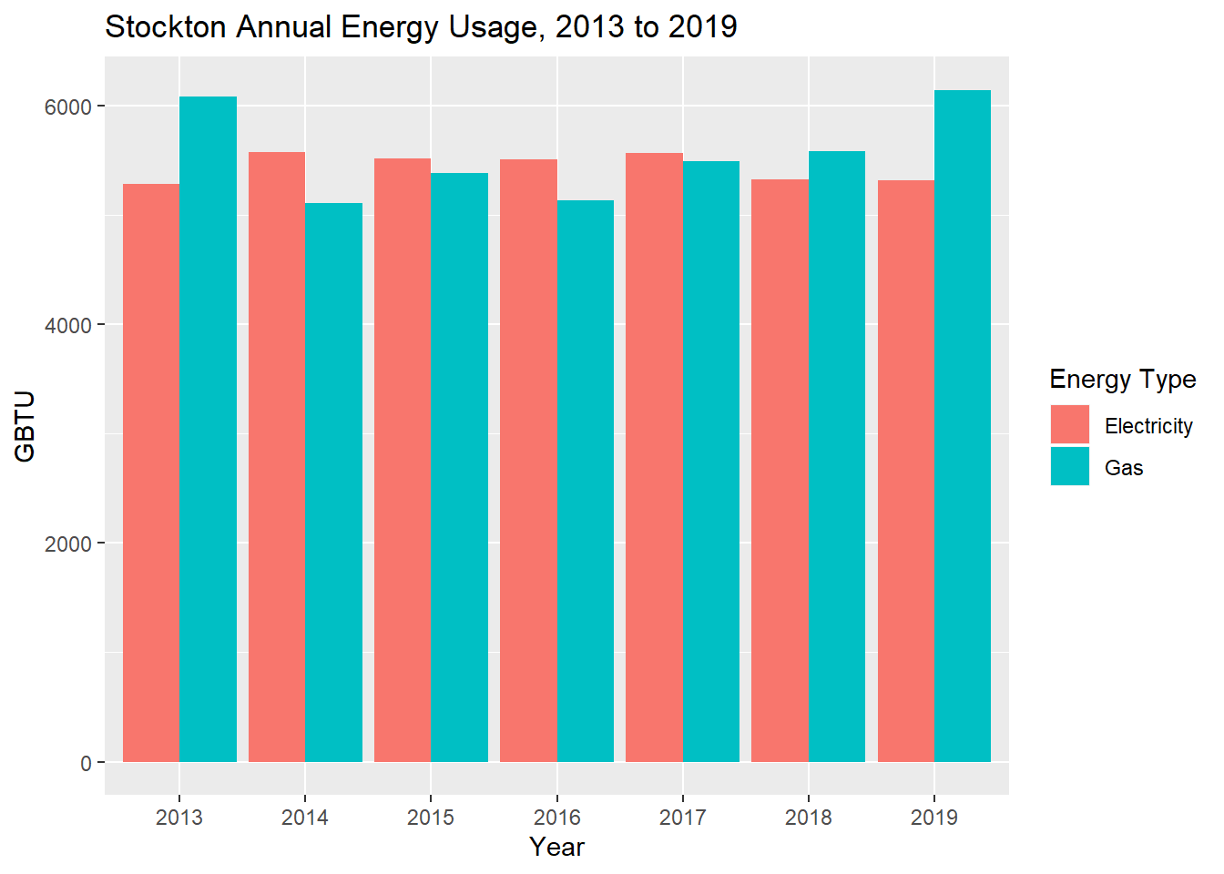
Figure 2.33: Stockton annual residential and commercial energy usage, 2013 to 2019, in kBTU. Data from PG&E.
\(~\)
ggplot(
  summary_TCO2E_average,
  aes(
    x = as.factor(YEAR),
    y = TOTALTCO2E
  )
) +
  geom_bar(stat = "identity", aes(fill = ENERGYTYPE), position = "dodge") +
  labs(x = "Year", y = "tCO2e", title = "Stockton Annual Energy Usage, 2013 to 2019") +
  scale_fill_discrete(name="Energy Type",labels = c("Electricity","Gas"))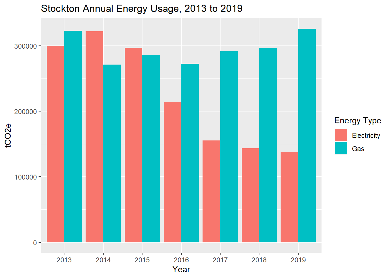
Figure 2.34: Stockton annual residential and commercial energy usage, 2013 to 2019, in tCO2e. Data from PG&E.
\(~\)
The following graph plots monthly tCO2e for electricity vs. gas. The peaks in gas usage occur in January, corresponding to heating load, and the peaks in electricity usage occur in July, corresponding to cooling load, and overall decreasing as previously noted. As we’ll explore in a later section, electrification of air and water heating in buildings may be a particularly effective strategy to shift the peak gas consumption to less carbon-intensive electricity loads.
summary_TCO2E_monthly <-
  pge_data %>%
  filter(!CUSTOMERCLASS %in% c("EI","EA")) %>%
  mutate(
    ENERGYTYPE = substr(CUSTOMERCLASS,1,1),
    MONTH = paste0(as.character(YEAR),substr(as.character(round(MONTH/100,2)),2,4))
  ) %>%
  group_by(MONTH, ENERGYTYPE) %>%
  summarize_at(
    vars(TOTALKBTU,TOTALTCO2E,TOTALCUSTOMERS),
    sum,
    na.rm=T
  ) %>%
  ungroup() %>%
  mutate(
    MONTH =
      as.Date(
        paste0(
          gsub(
            "\\.",
            "\\/",
            ifelse(
              nchar(MONTH) == 6,
              paste0(MONTH,"0"),
              MONTH
            )
          ),
          "/01"
        )
      )
  )

ggplot(
  summary_TCO2E_monthly,
  aes(
    x = MONTH,
  )
) +
  geom_line(
    aes(
      y = TOTALTCO2E,
      color = ENERGYTYPE
    )
  ) +
  labs(x = "Month", y = "tCO2e", title = "Stockton Monthly Energy Usage, 2013 to 2019") +
  scale_color_manual(
    name= "Energy Type",
    values = c("blue","red"),
    labels = c("Electricity","Gas")
  ) +
  scale_x_date(
    name = 'Year',
    date_breaks = '1 year',
    date_labels = '%Y'
  )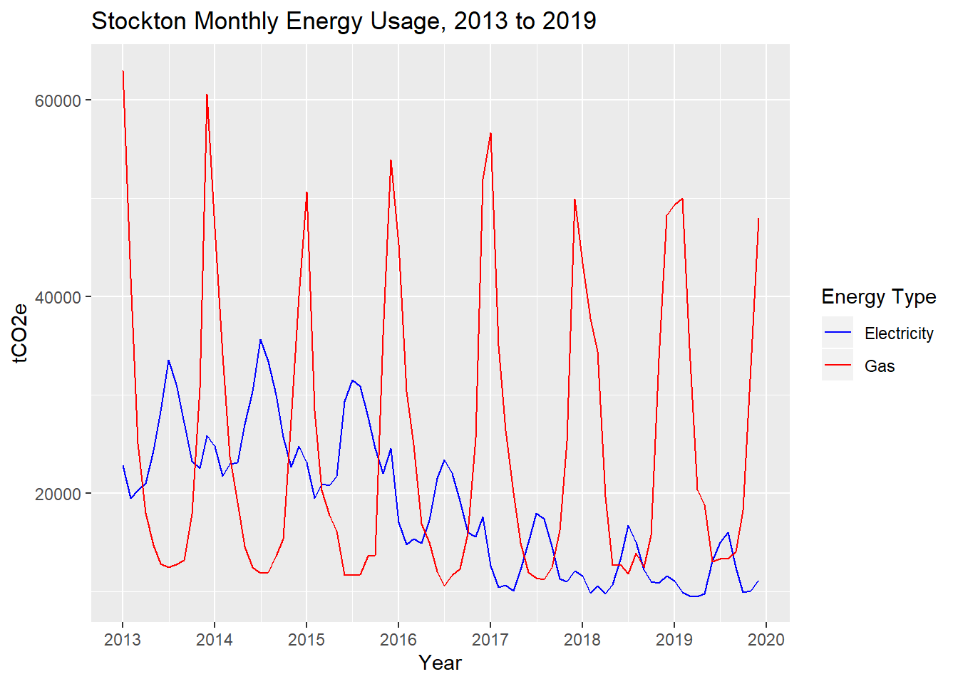
Figure 2.35: Stockton monthly residential and commercial energy usage, 2013 to 2019, in tCO2e. Data from PG&E.
\(~\)
Note that heating and cooling loads, which appear to contribute to significant seasonal variation within years, is also heavily dependent on the specific weather in any given year, typically measured in heating degree days (HDDs) and cooling degree days (CDDs). A more accurate comparison of annual energy consumption would control for change in HDDs and CDDs year-to-year; a more accurate forecasting of energy consumption into the future would also factor in climate model predictions of future HDDs and CDDs.
We used the Cal-Adapt Degree Day tool to collect HDDs and CDDs for Stockton from 2010 to 2018, and on to 2040, using the average simulation (CanESM2) under the Representative Concentration Pathway (RCP) 4.5 scenario (in which global GHG emissions peak around 2040, then decline). The graph below shows the data from Cal-Adapt, as well as linear trendlines, with a clear overall upwards trend for CDDs (meaning that temperatures are rising and more cooling power is needed), and a clear overall downwards trend for HDDs.
hdd <-
  read_csv("C:/Users/derek/Google Drive/City Systems/Stockton Green Economy/hdd.csv") %>%
  transmute(
    YEAR = year,
    hdd = degree_days
  )
cdd <-
  read_csv("C:/Users/derek/Google Drive/City Systems/Stockton Green Economy/cdd.csv") %>%
  filter(model == "CanESM2") %>%
  transmute(
    YEAR = year,
    cdd = degree_days
  )

hdd %>%
  filter(YEAR >= 2010 & YEAR <=2040) %>%
  left_join(cdd, by = "YEAR") %>%
  ggplot(
    aes(
      x = YEAR
    )
  ) +
  geom_line(
    aes(
      y = hdd,
      colour = "Heating",
      linetype = "Cal-Adapt"
    )
  ) +
  geom_smooth(
    aes(
      y = hdd,
      colour = "Heating",
      linetype = "Trendline"
    ),
    method = lm,
    se = FALSE
  ) +
  geom_line(
    aes(
      y = cdd,
      colour = "Cooling",
      linetype = "Cal-Adapt"
    )
  ) +
  geom_smooth(
    aes(
      y = cdd,
      colour = "Cooling",
      linetype = "Trendline"
    ),
    method = lm,
    se = FALSE
  ) +
  geom_vline(aes(xintercept = 2018), color = "dark grey") +
  annotate("text",label= "Historical\n", color = "dark grey", x=2018, y=2600, angle = 90, size=4) +
  annotate("text",label= "\nForecast", color = "dark grey", x=2018, y=2600, angle = 90, size=4) +
  scale_colour_manual(values = c("red","blue")) +
  scale_linetype_manual(values = c("solid","dotted")) +
  labs(title = "Stockton Heating and Cooling Degree Days", y = "Degree Days", colour = "")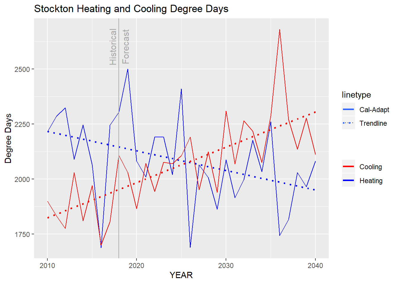
Figure 2.36: Stockton heating and cooling degree days under RCP 4.5 scenario, 2010 to 2040. Data from Cal-Adapt.
\(~\)
The following table shows historical 2013-2018 annual energy usage per capita (residents for residential energy, jobs for commercial energy) per degree day (HDDs for gas, CDDs for electricity), and the graph that follows shows these four energy use factors with downward trends. This may be through a combination of changing building energy efficiency as well as changing building utilization (e.g. more or less space per occupant), though we don’t have the data to be able to separate these two factors.
summary_TCO2E_norm <-
  pge_data %>%
  filter(!CUSTOMERCLASS %in% c("EI","EA")) %>%
  group_by(ZIPCODE, CUSTOMERCLASS, YEAR) %>%
  summarize(
    TOTALKBTU = sum(TOTALKBTU, na.rm=T),
    TOTALTCO2E = sum(TOTALTCO2E, na.rm=T),
    TOTALCUSTOMERS = mean(TOTALCUSTOMERS, na.rm=T)
  ) %>%
  group_by(CUSTOMERCLASS, YEAR) %>%
  summarize_at(
    vars(TOTALKBTU,TOTALTCO2E,TOTALCUSTOMERS),
    sum,
    na.rm=T
  ) %>%
  left_join(hdd, by = "YEAR") %>%
  left_join(cdd, by = "YEAR") %>%
  left_join(pop_stockton, by = c("YEAR" = "year")) %>%
  left_join(jobs_stockton, by = c("YEAR" = "year"))

summary_TCO2E_norm_ER <-
  summary_TCO2E_norm %>%
  filter(CUSTOMERCLASS == "ER") %>%
  mutate(
    KBTU_res_cdd =
      TOTALKBTU/PopulationStockton/cdd,
    TCO2E_res_cdd =
      TOTALTCO2E/PopulationStockton/cdd
  )

summary_TCO2E_norm_GR <-
  summary_TCO2E_norm %>%
  filter(CUSTOMERCLASS == "GR") %>%
  mutate(
    KBTU_res_hdd =
      TOTALKBTU/PopulationStockton/hdd,
    TCO2E_res_hdd =
      TOTALTCO2E/PopulationStockton/hdd
  )

summary_TCO2E_norm_EC <-
  summary_TCO2E_norm %>%
  filter(CUSTOMERCLASS == "EC") %>%
  mutate(
    KBTU_job_cdd =
      TOTALKBTU/Jobs/cdd,
    TCO2E_job_cdd =
      TOTALTCO2E/Jobs/cdd
  )

summary_TCO2E_norm_GC <-
  summary_TCO2E_norm %>%
  filter(CUSTOMERCLASS == "GC") %>%
  mutate(
    KBTU_job_hdd =
      TOTALKBTU/Jobs/hdd,
    TCO2E_job_hdd =
      TOTALTCO2E/Jobs/hdd
  )

summary_TCO2E_norm_all <-
  summary_TCO2E_norm_ER %>%
  ungroup() %>%
  transmute(
    Year = YEAR,
    `Heating Degree Days` = prettyNum(round(hdd,-2),big.mark=","),
    `Cooling Degree Days` = prettyNum(round(cdd,-2),big.mark=","),
    Residents = prettyNum(round(PopulationStockton,-3),big.mark=","),
    Jobs = prettyNum(round(Jobs,-3),big.mark=","),
    `Residential Electricity, kBTU/resident/CDD` = round(KBTU_res_cdd,1)
  ) %>%
  mutate(
    `Residential Gas, kBTU/resident/HDD` = round(summary_TCO2E_norm_GR$KBTU_res_hdd,1),
    `Commercial Electricity, kBTU/job/CDD` = round(summary_TCO2E_norm_EC$KBTU_job_cdd,1),
    `Commercial Gas, kBTU/job/HDD` = round(summary_TCO2E_norm_GC$KBTU_job_hdd,1)
  )

kable(
  summary_TCO2E_norm_all,
  booktabs = TRUE,
  caption = 'Stockton annual energy use per capita per degree-day, 2013 to 2018.'
) %>%
  kable_styling() %>%
scroll_box(width = "100%")| Year | Heating Degree Days | Cooling Degree Days | Residents | Jobs | Residential Electricity, kBTU/resident/CDD | Residential Gas, kBTU/resident/HDD | Commercial Electricity, kBTU/job/CDD | Commercial Gas, kBTU/job/HDD |
|---|---|---|---|---|---|---|---|---|
| 2013 | 2,100 | 2,000 | 298,000 | 106,000 | 4.7 | 7.7 | 11.5 | 5.7 |
| 2014 | 2,200 | 1,800 | 302,000 | 107,000 | 5.2 | 5.9 | 14.1 | 4.7 |
| 2015 | 2,100 | 2,000 | 306,000 | 114,000 | 4.7 | 6.7 | 12.1 | 4.9 |
| 2016 | 1,700 | 1,700 | 307,000 | 116,000 | 5.3 | 8.0 | 13.9 | 5.0 |
| 2017 | 2,200 | 1,800 | 310,000 | 117,000 | 5.2 | 6.2 | 12.6 | 4.3 |
| 2018 | 2,300 | 2,100 | 311,000 | 118,000 | 4.1 | 6.1 | 10.5 | 4.4 |
| 2019 | 2,500 | 2,000 | NA | NA | NA | NA | NA | NA |
\(~\)
summary_TCO2E_norm_all %>%
  filter(Year != 2019) %>%
  ggplot(
    aes(
      x = Year
    )
  ) +
  geom_line(
    aes(
      y = `Residential Electricity, kBTU/resident/CDD`,
      colour = "Residential Electricity\n(kBTU/resident/CDD)",
      linetype = "Historical"
    )
  ) +
  geom_smooth(
    aes(
      y = `Residential Electricity, kBTU/resident/CDD`,
      colour = "Residential Electricity\n(kBTU/resident/CDD)",
      linetype = "Trendline"
    ),
    method = lm,
    se = FALSE
  )+
  geom_line(
    aes(
      y = `Residential Gas, kBTU/resident/HDD`,
      colour = "Residential Gas\n(kBTU/resident/HDD)",
      linetype = "Historical"
    )
  ) +
  geom_smooth(
    aes(
      y = `Residential Gas, kBTU/resident/HDD`,
      colour = "Residential Gas\n(kBTU/resident/HDD)",
      linetype = "Trendline"
    ),
    method = lm,
    se = FALSE
  ) +
  geom_line(
    aes(
      y = `Commercial Electricity, kBTU/job/CDD`,
      colour = "Commercial Electricity\n(kBTU/job/CDD)",
      linetype = "Historical"
    )
  ) +
  geom_smooth(
    aes(
      y = `Commercial Electricity, kBTU/job/CDD`,
      colour = "Commercial Electricity\n(kBTU/job/CDD)",
      linetype = "Trendline"
    ),
    method = lm,
    se = FALSE
  ) +
  geom_line(
    aes(
      y = `Commercial Gas, kBTU/job/HDD`,
      colour = "Commercial Gas\n(kBTU/job/HDD)",
      linetype = "Historical"
    )
  ) +
  geom_smooth(
    aes(
      y = `Commercial Gas, kBTU/job/HDD`,
      colour = "Commercial Gas\n(kBTU/job/HDD)",
      linetype = "Trendline"
    ),
    method = lm,
    se = FALSE
  ) +
  scale_colour_manual(values = c("red","blue","orange", "green")) +
  scale_linetype_manual(values = c("solid","dotted")) +
  labs(title = "Stockton Energy Use per Capita per Degree-Day", y = "kBTU/cap/degree-day", colour = "Energy Factor", linetype = "Data Type")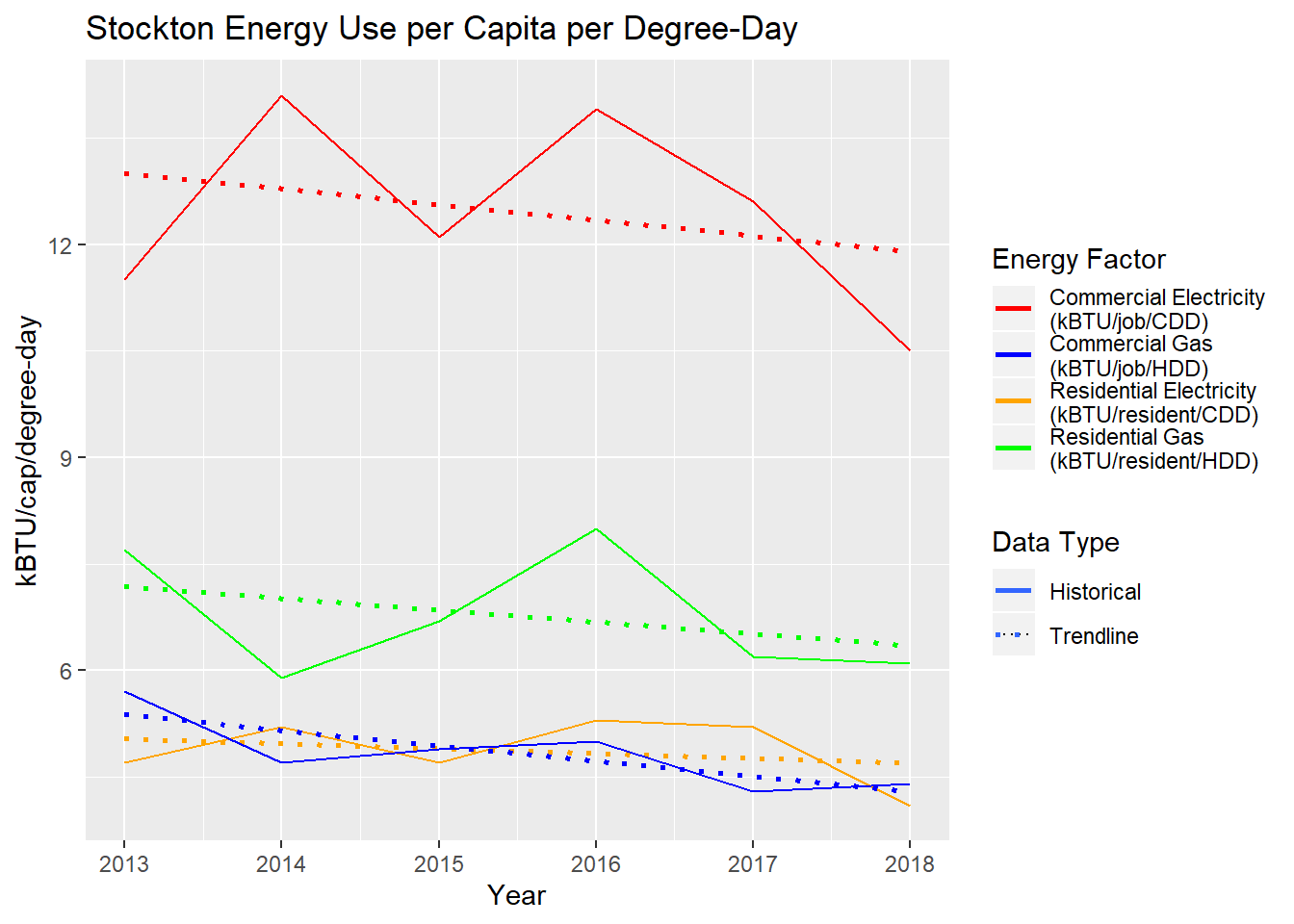
Figure 2.37: Stockton annual energy use per capita per degree-day, 2013 to 2018.
\(~\)
A full forecast of energy usage will also depend on predicted changes in resident and job populations, which will lead to more buildings and more energy used in buildings, predicted changes in building energy efficiency and utilization, predicted changes in weather, and many other factors that are outside the scope of this analysis. One last available dataset to incorporate into our understanding of energy use relates to buildings.