2.1 Population and Jobs
The following analysis first processes population and jobs data at the County (SJC) level, where it is more readily available, followed by estimations at the City level.
2.1.1 County-level Analysis
The following datasets were collected for SJC:
- Total Population, American Communities Survey, 1-Yr Estimates, 2010-2018
- Population projections for US counties, 2020-2100
- Longitudinal Employer-Household Dynamics Origin-Destination Employment Statistics, 2010-2017, available at the block level
A few notes on methodology and assumptions:
- From the ACS, we collected Total Population, Total Population 16 and Older, Total Employed Residents (16+), and Unemployment Rate (for 16+). In order to forecast the future number of employed residents, which would then be used to forecast the future number of jobs, we chose to perform a linear regression on employment rate projecting to 2040, given that the unemployment rate was significantly more variable from 2010-2018.
- Population projections come from a study published in Nature in 2019. The specific methodology is beyond the scope of this project to unpack. What’s notable is that five different projections were made by the author based on diferent “potential futures involving various growth policies, fossil-fuel usage, mitigation policies (i.e. emission reductions), adaptation policies (i.e. deployment of flood defenses), and population change”. We used the “Middle of the road” projection.
- Projections from the above study were available in 5-year age groups. While the total population projection is directly used in the final table below for SJC, Population of 15+ was also collected which was multiplied by the previously projected Employment Rate (#1) to forecast total Employed Residents. Note that given data limitations we have a discontinuity between Population 16+ data from 2010-2018 and Population 15+ data from 2020-2040. We assume this difference is negligible for the purposes of our analysis, but it would have the effect of overestimating job count.
- From LODES we collected “Primary Jobs” at the block group level and aggregated all jobs for block groups in SJC. These are meant to match the number of individual workers in a region. We also compared this number to the number of employees provided by the Quarterly Workforce Indicators dataset and the number of nonemployer establishments in the Nonemployer Statistics dataset. The LODES Primary Jobs number was higher than the QWI Employee count but lower than the QWI Employee count plus Nonemployer Establishments count, which seems to make sense (since an individual could operate multiple nonemployer establishments).
- We calculated J/ER for 2010-2018 by dividing total Jobs by Employed Residents. Then, we chose to perform a linear regression on J/ER ratio projecting to 2040, and multiplied this by our projected Employed Residents (#3) to forecast total Jobs.
ca_counties <- counties("CA", cb = TRUE)
ca_tracts <- tracts("CA", cb = TRUE)
ca_bgs <- block_groups("CA", cb = TRUE)

county_neighbors <-
  ca_counties %>%
  filter(NAME %in% c(
    "San Joaquin",
    "Alameda",
    "Sacramento",
    "Santa Clara",
    "Stanislaus",
    "Contra Costa",
    "San Francisco",
    "San Mateo",
    "Solano",
    "Fresno",
    "Placer",
    "Yolo",
    "Sonoma",
    "Merced",
    "Monterey"
  ))

pop_sjc <- data.frame(matrix(ncol=3,nrow=0))
colnames(pop_sjc) <- c("Population","Population15andolder","year")

for(year in 2010:2018){

  temp <-
    getCensus(
      name = "acs/acs1",
      vintage = year,
      vars = c("B01003_001E"),
      region = "county:077",
      regionin = "state:06"
    ) %>%
    mutate(
      Population = B01003_001E,
      year = year
    ) %>%
    dplyr::select(
      Population,
      year
    )

  pop_sjc<- rbind(pop_sjc,temp)

}

sjc_projection <-
  read_csv("C:/Users/derek/Google Drive/City Systems/Stockton Green Economy/SSP_asrc_STATEfiles/DATA-PROCESSED/SPLITPROJECTIONS/CA.csv") %>%
  filter(COUNTY == "077") %>%
  group_by(YEAR) %>%
  summarize(
    Population = sum(SSP2),
    Population15andOlder = sum(SSP2[which(AGE > 3)])
  ) %>%
  filter(YEAR %in% c(2020,2025,2030,2035,2040)) %>%
  dplyr::select(Population, Population15andOlder, year = YEAR)

pop_sjc_w_projection <-
  bind_rows(pop_sjc,sjc_projection)

emp_sjc <- data.frame(matrix(ncol=2,nrow=0))
colnames(emp_sjc) <- c("EmployedResidents","year")

for(year in 2010:2018){

  temp <-
    getCensus(
      name = "acs/acs1/subject",
      vintage = year,
      vars = c("S2301_C01_001E","S2301_C03_001E","S2301_C04_001E"),
      region = "county:077",
      regionin = "state:06"
    ) %>%
    mutate(
      Population16andOlder = S2301_C01_001E,
      PercEmployedResidents = S2301_C03_001E,
      EmployedResidents = PercEmployedResidents/100*Population16andOlder,
      UnemploymentRate = S2301_C04_001E,
      year = year
    ) %>%
    dplyr::select(
      Population16andOlder,
      PercEmployedResidents,
      EmployedResidents,
      UnemploymentRate,
      year
    )

  emp_sjc<- rbind(emp_sjc,temp)

}

pop_emp_sjc_w_projection <-
  pop_sjc_w_projection %>%
  left_join(emp_sjc, by = "year") %>%
  mutate(
    PercEmployedResidents = ifelse(
      !is.na(PercEmployedResidents),
      PercEmployedResidents,
      lm(
        formula = `PercEmployedResidents`[1:9] ~ year[1:9]
      )$coefficients[1]+
        lm(
          formula = `PercEmployedResidents`[1:9] ~ year[1:9]
        )$coefficients[2]*year
    ),
    EmployedResidents = ifelse(!is.na(EmployedResidents),EmployedResidents,Population15andOlder*PercEmployedResidents/100)
  )

# sjc_wac <-
#   2010:2017 %>%
#   map(function(year){
#     ca_wac <-
#       grab_lodes(
#         state = "ca",
#         year = year,
#         lodes_type = "wac",
#         job_type = "JT01",
#         segment = "S000",
#         state_part = "main",
#         agg_geo = "bg"
#       )
#
#     temp <-
#       ca_wac %>%
#       filter(substr(w_bg,1,5) == "06077")
#
#     return(temp)
#   }) %>%
#   rbindlist()
#
# save(sjc_wac, file = "C:/Users/derek/Google Drive/City Systems/Stockton Green Economy/sjc_wac.Rdata")
load("C:/Users/derek/Google Drive/City Systems/Stockton Green Economy/sjc_wac.Rdata")

jobs_sjc <-
  sjc_wac %>%
  group_by(year) %>%
  summarize(Jobs = sum(C000))

#Add 2018 jobs projection
jobs_sjc[9,1] <- 2018
jobs_sjc[9,2] <-
  lm(formula = jobs_sjc$Jobs[1:8] ~ jobs_sjc$year[1:8])$coefficients[1]+
  lm(formula = jobs_sjc$Jobs[1:8] ~ jobs_sjc$year[1:8])$coefficients[2]*2018

pop_jobs_sjc_w_projection <-
  pop_emp_sjc_w_projection %>%
  left_join(jobs_sjc, by = "year") %>%
  mutate(
    ratio = ifelse(
      !is.na(Jobs),
      Jobs/EmployedResidents,
      lm(
        formula = Jobs[1:9]/EmployedResidents[1:9] ~ year[1:9]
      )$coefficients[1]+
        lm(
          formula = Jobs[1:9]/EmployedResidents[1:9] ~ year[1:9]
        )$coefficients[2]*year
    ),
    Jobs = ifelse(!is.na(Jobs),Jobs,EmployedResidents*ratio)
  ) %>%
  transmute(
    Year = year,
    Population = Population,
    Jobs = Jobs,
    `Employed Residents` = EmployedResidents,
    `J/ER Ratio` = ratio,
    `Percent Employed Residents` = PercEmployedResidents,
    `Percent Unemployment` = UnemploymentRate
  )

pop_jobs_sjc_w_projection_table <-
  pop_jobs_sjc_w_projection %>%
  transmute(
    Year = Year,
    Population = prettyNum(round(Population,-3),big.mark=","),
    Jobs = prettyNum(round(Jobs,-3),big.mark=","),
    `Employed Residents` = prettyNum(round(`Employed Residents`,-3),big.mark=","),
    `J/ER Ratio` = round(`J/ER Ratio`,2),
    `Percent Employed Residents` = paste0(round(`Percent Employed Residents`),"%"),
    `Percent Unemployment` = ifelse(is.na(`Percent Unemployment`),"NA",paste0(round(`Percent Unemployment`),"%"))
  )

# save(pop_jobs_sjc_w_projection, file = "C:/Users/derek/Google Drive/City Systems/Stockton Green Economy/pop_jobs_sjc_w_projection.Rdata")

kable(
  pop_jobs_sjc_w_projection_table,
  booktabs = TRUE,
  caption = 'Historical population and job counts for San Joaquin County 2010-2017, followed by projections to 2040.'
) %>%
  kable_styling() %>%
scroll_box(width = "100%")| Year | Population | Jobs | Employed Residents | J/ER Ratio | Percent Employed Residents | Percent Unemployment |
|---|---|---|---|---|---|---|
| 2010 | 688,000 | 185,000 | 265,000 | 0.70 | 52% | 17% |
| 2011 | 696,000 | 184,000 | 264,000 | 0.70 | 51% | 18% |
| 2012 | 703,000 | 187,000 | 270,000 | 0.69 | 52% | 16% |
| 2013 | 704,000 | 192,000 | 278,000 | 0.69 | 52% | 13% |
| 2014 | 716,000 | 197,000 | 290,000 | 0.68 | 54% | 11% |
| 2015 | 726,000 | 212,000 | 293,000 | 0.72 | 53% | 11% |
| 2016 | 734,000 | 220,000 | 306,000 | 0.72 | 55% | 9% |
| 2017 | 745,000 | 226,000 | 314,000 | 0.72 | 56% | 6% |
| 2018 | 753,000 | 230,000 | 326,000 | 0.70 | 57% | 6% |
| 2020 | 763,000 | 247,000 | 343,000 | 0.72 | 58% | NA |
| 2025 | 797,000 | 285,000 | 388,000 | 0.74 | 61% | NA |
| 2030 | 829,000 | 324,000 | 432,000 | 0.75 | 65% | NA |
| 2035 | 859,000 | 363,000 | 474,000 | 0.76 | 68% | NA |
| 2040 | 886,000 | 403,000 | 518,000 | 0.78 | 72% | NA |
\(~\)
The figure below shows the J/ER ratio projected out to 2040, reaching a high of 0.78. This is not particularly high (given our goal of surpassing 1). There is certainly room for improvement through proactive economic development strategies.
ggplot(pop_jobs_sjc_w_projection, aes(x = Year)) +
  geom_line(aes(y = `J/ER Ratio`), size=2, colour = "forest green") +
  geom_vline(aes(xintercept = 2018), color = "dark grey") +
  annotate("text",label= "Data Available\n", color = "dark grey", x=2018, y=.75, angle = 90, size=4) +
  annotate("text",label= "\nForecast", color = "dark grey", x=2018, y=.75, angle = 90, size=4) +
  labs(title = "San Joaquin County, CA")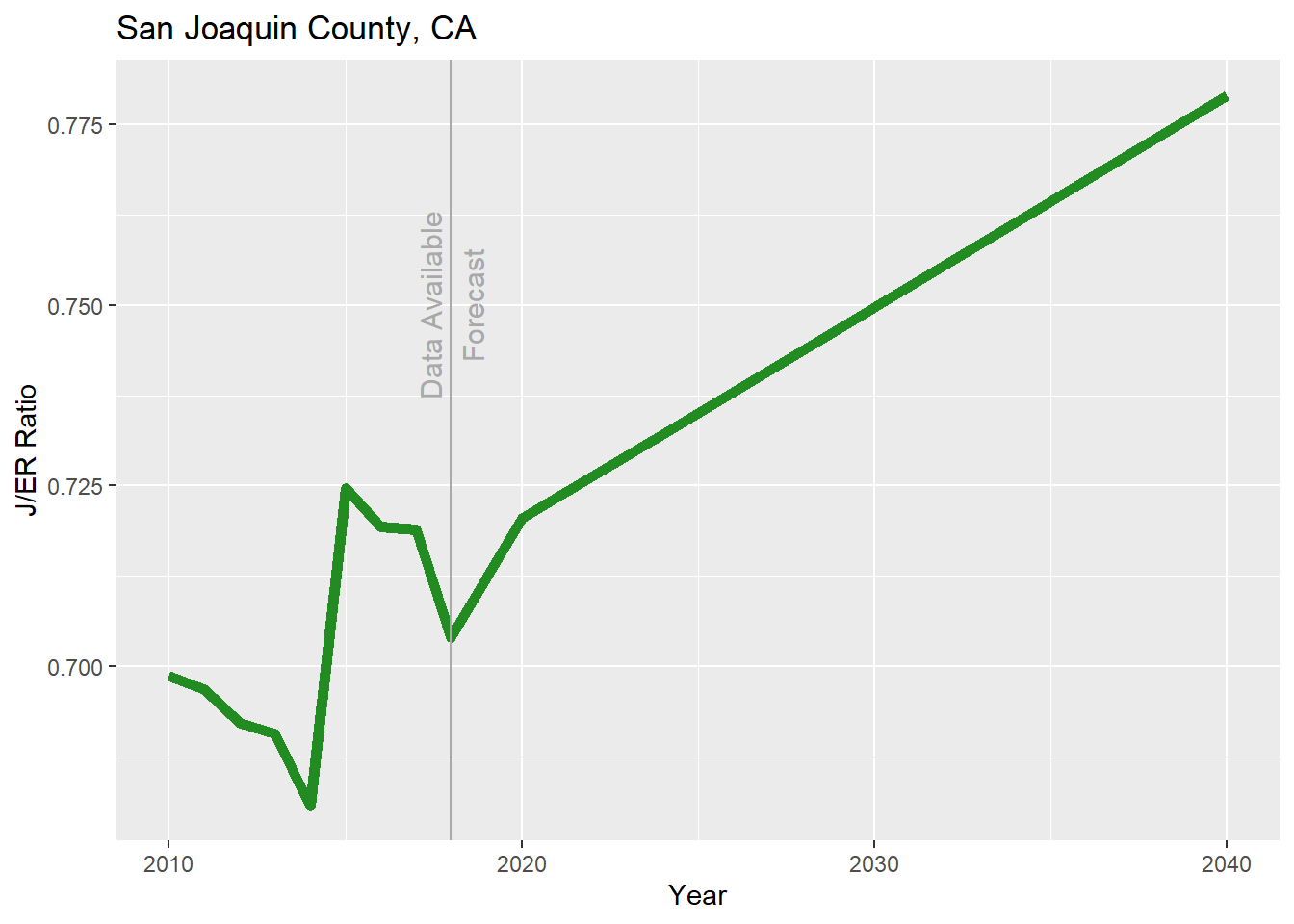
Figure 2.1: Historical Jobs to Employed Residents Ratio for San Joaquin County 2010-2018, followed by projections to 2040.
\(~\)
ggplot(pop_jobs_sjc_w_projection, aes(x = Year)) +
  geom_line(aes(y = `Employed Residents`/100000, colour = "Employed Residents"), size = 2) +
  geom_line(aes(y = Jobs/100000, colour = "Jobs"), size = 2) +
  geom_line(aes(y = Population/100000, colour = "Population"), size = 2) +
  geom_vline(aes(xintercept = 2018), color = "dark grey") +
  annotate("text",label= "Data Available\n", color = "dark grey", x=2018, y=5, angle = 90, size=4) +
  annotate("text",label= "\nForecast", color = "dark grey", x=2018, y=5, angle = 90, size=4) +
  scale_colour_manual(values = c("purple","blue","red")) +
  labs(title = "San Joaquin County, CA", y = "Count (100,000s)", colour = "")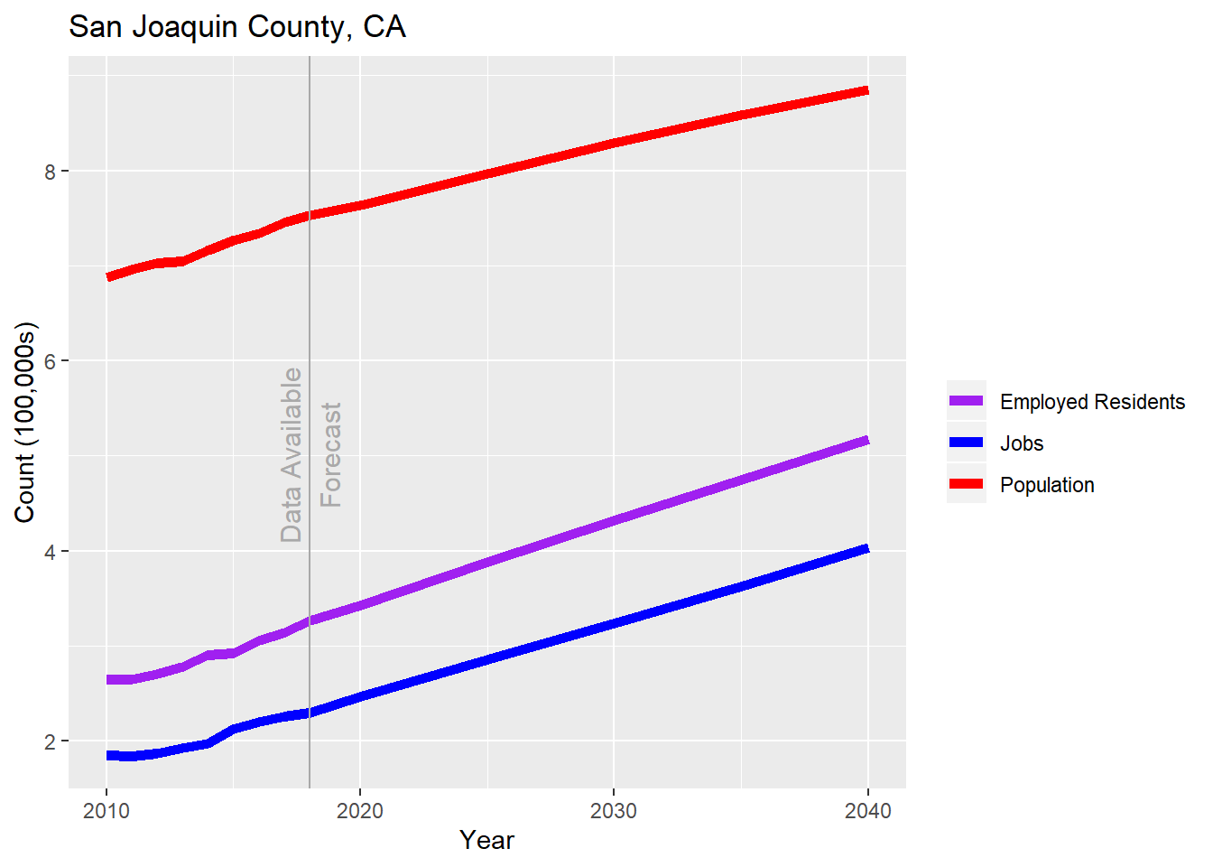
Figure 2.2: Historical population, employed residents, and jobs for San Joaquin County 2010-2018, followed by projections to 2040.
\(~\)
The following figure compares the J/ER ratio for SJC and its neighboring counties since 2010. SJC is toward the lower end of the group. It appears that all of these counties are stagnant or decreasing in this metric, and are all “bedroom counties” in the sense of being net exporters of workers during the day.
# county_jer <- NULL
#
# for(year in 2010:2017){
#
#   ca_wac <-
#     grab_lodes(
#       state = "ca",
#       year = year,
#       lodes_type = "wac",
#       job_type = "JT01",
#       segment = "S000",
#       state_part = "main",
#       agg_geo = "tract"
#     )
#
#   for(county in county_neighbors$COUNTYFP){
#
#      temp <-
#       getCensus(
#         name = "acs/acs1/subject",
#         vintage = year,
#         vars = c("S2301_C01_001E","S2301_C03_001E","S2301_C04_001E"),
#         region = paste0("county:",county),
#         regionin = "state:06"
#       ) %>%
#       mutate(
#         Population16andOlder = S2301_C01_001E,
#         PercEmployedResidents = S2301_C03_001E,
#         EmployedResidents = round( PercEmployedResidents/100*Population16andOlder),
#         Year = year,
#         Jobs =
#           ca_wac %>%
#           filter(substr(w_tract,3,5) == county) %>%
#           pull(C000) %>%
#           sum(na.rm=T),
#         County = county_neighbors[which(county_neighbors$COUNTYFP == county),]$NAME,
#       ) %>%
#       dplyr::select(
#         County,
#         Year,
#         Jobs,
#         EmployedResidents
#       )
#
#     county_jer<- rbind(county_jer,temp)
#   }
# }
#
# save(county_jer,file="C:/Users/derek/Google Drive/City Systems/Stockton Green Economy/county_jer.Rdata")
load("C:/Users/derek/Google Drive/City Systems/Stockton Green Economy/county_jer.Rdata")

county_jer %>%
  filter(County %in% c("San Joaquin","Stanislaus","Alameda","Sacramento","Fresno","Solano","Contra Costa")) %>%
  ggplot(
    aes(
      x = Year,
      y = Jobs/EmployedResidents,
      colour = County
    )
  ) +
  geom_line()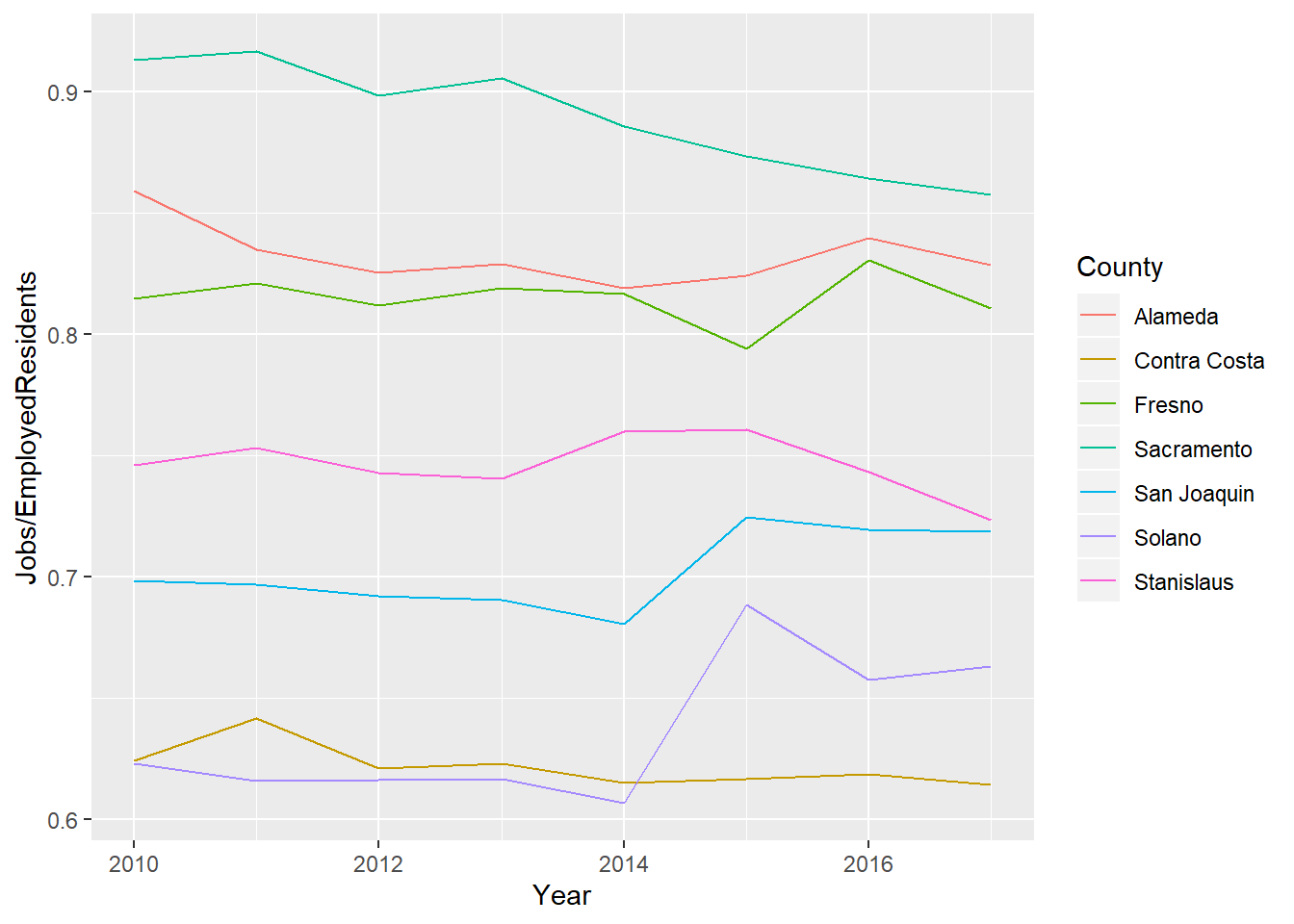
Figure 2.3: Comparison of Jobs to Employment Ratio for different counties, 2010-2017.
\(~\)
The Quarterly Workforce Indicators dataset also illustrates the number and average quarterly earnings of jobs in different sub-level NAICS industry sectors (228 total). The table below is sorted by sectors with the most jobs in SJC.
label_industry <-
  read_csv("C:/Users/derek/Google Drive/City Systems/Stockton Green Economy/label_industry.csv")

# qwi_sjc <- data.frame(matrix(ncol=5,nrow=0))
# colnames(qwi_sjc) <- c("year","industry","label","EmpS","EarnS")
#
# for(years in 2010:2018){
#   qwi<-
#     getCensus(
#       name = "timeseries/qwi/sa",
#       region = "county:077",
#       regionin = "state:06",
#       vars = c("EmpS","EarnS","industry","ind_level"),
#       time = years
#     ) %>%
#     filter(ind_level == 4) %>%
#     mutate(
#       year = substr(time,1,4)
#     ) %>%
#     left_join(label_industry, by= "industry") %>%
#     group_by(year,industry,label) %>%
#     summarize(
#       EmpS = round(mean(as.numeric(EmpS), na.rm = TRUE),0),
#       EarnS = round(mean(as.numeric(EarnS), na.rm = TRUE),0)
#     ) %>%
#     filter(!is.na(EmpS) & EmpS != 0)
#
#   qwi_sjc<-
#     bind_rows(qwi_sjc,qwi)
# }
#
# save(qwi_sjc, file = "C:/Users/derek/Google Drive/City Systems/Stockton Green Economy/qwi_sjc.Rdata")
load("C:/Users/derek/Google Drive/City Systems/Stockton Green Economy/qwi_sjc.Rdata")

qwi_sjc_18 <-
  qwi_sjc %>%
  filter(year == 2018) %>%
  arrange(desc(EmpS)) %>%
  transmute(
    Label = label,
    Jobs = prettyNum(round(EmpS,-2),big.mark=","),
    `Average Quarterly Earnings` = paste0("$",prettyNum(round(EarnS,-2),big.mark=","))
  )

kable(
  qwi_sjc_18,
  booktabs = TRUE,
  caption = 'Job counts and earnings by NAICS industry sector for San Joaquin County 2018.'
) %>%
  kable_styling() %>%
scroll_box(width = "100%", height = "500px")| Label | Jobs | Average Quarterly Earnings |
|---|---|---|
| Elementary and Secondary Schools | 17,100 | $4,300 |
| Warehousing and Storage | 15,300 | $3,300 |
| Restaurants and Other Eating Places | 14,100 | $1,700 |
| Individual and Family Services | 7,300 | $1,200 |
| General Medical and Surgical Hospitals | 7,100 | $6,500 |
| Justice, Public Order, and Safety Activities | 4,900 | $6,600 |
| General Freight Trucking | 4,600 | $4,800 |
| General Merchandise Stores, including Warehouse Clubs and Supercenters | 4,300 | $2,900 |
| Grocery and Related Product Merchant Wholesalers | 4,200 | $4,500 |
| Support Activities for Crop Production | 4,000 | $2,800 |
| Employment Services | 3,700 | $2,900 |
| Grocery Stores | 3,400 | $2,700 |
| Executive, Legislative, and Other General Government Support | 3,300 | $6,200 |
| Nursing Care Facilities (Skilled Nursing Facilities) | 3,100 | $3,100 |
| Offices of Physicians | 3,000 | $6,700 |
| Fruit and Tree Nut Farming | 2,900 | $3,000 |
| Building Equipment Contractors | 2,500 | $5,500 |
| Services to Buildings and Dwellings | 2,500 | $2,700 |
| Outpatient Care Centers | 2,300 | $9,900 |
| Colleges, Universities, and Professional Schools | 2,300 | $4,500 |
| Beverage Manufacturing | 2,200 | $4,200 |
| Administration of Human Resource Programs | 2,200 | $6,100 |
| Automotive Repair and Maintenance | 2,100 | $3,400 |
| Management of Companies and Enterprises | 2,100 | $4,800 |
| Building Material and Supplies Dealers | 1,900 | $3,100 |
| Agencies, Brokerages, and Other Insurance Related Activities | 1,900 | $6,400 |
| Building Finishing Contractors | 1,900 | $3,600 |
| Automobile Dealers | 1,800 | $4,900 |
| Foundation, Structure, and Building Exterior Contractors | 1,800 | $4,100 |
| Other Amusement and Recreation Industries | 1,800 | $2,500 |
| Specialized Freight Trucking | 1,800 | $4,800 |
| Investigation and Security Services | 1,700 | $2,800 |
| Offices of Dentists | 1,700 | $3,800 |
| Health and Personal Care Stores | 1,500 | $3,800 |
| Vocational Rehabilitation Services | 1,500 | $5,000 |
| Continuing Care Retirement Communities and Assisted Living Facilities for the Elderly | 1,400 | $2,500 |
| Machinery, Equipment, and Supplies Merchant Wholesalers | 1,300 | $5,600 |
| Depository Credit Intermediation | 1,300 | $8,000 |
| Couriers and Express Delivery Services | 1,200 | $2,600 |
| Clothing Stores | 1,200 | $1,800 |
| Automotive Parts, Accessories, and Tire Stores | 1,200 | $3,200 |
| Residential Building Construction | 1,200 | $4,100 |
| Other Specialty Trade Contractors | 1,100 | $5,100 |
| Administration of Economic Programs | 1,100 | $6,700 |
| Professional and Commercial Equipment and Supplies Merchant Wholesalers | 1,100 | $8,400 |
| Offices of Other Health Practitioners | 1,100 | $3,200 |
| Architectural and Structural Metals Manufacturing | 1,100 | $5,700 |
| Motor Vehicle and Motor Vehicle Parts and Supplies Merchant Wholesalers | 1,100 | $4,800 |
| Department Stores | 1,100 | $2,000 |
| Gasoline Stations | 1,100 | $2,200 |
| Cattle Ranching and Farming | 1,100 | $3,100 |
| Animal Slaughtering and Processing | 1,000 | $4,300 |
| Highway, Street, and Bridge Construction | 1,000 | $6,900 |
| Traveler Accommodation | 1,000 | $2,200 |
| Other Wood Product Manufacturing | 1,000 | $4,300 |
| Fruit and Vegetable Preserving and Specialty Food Manufacturing | 1,000 | $4,500 |
| Vegetable and Melon Farming | 900 | $3,600 |
| Miscellaneous Nondurable Goods Merchant Wholesalers | 900 | $6,000 |
| Personal Care Services | 900 | $1,700 |
| Accounting, Tax Preparation, Bookkeeping, and Payroll Services | 900 | $4,400 |
| Management, Scientific, and Technical Consulting Services | 900 | $3,800 |
| Converted Paper Product Manufacturing | 900 | $5,200 |
| Child Day Care Services | 800 | $2,200 |
| Nonresidential Building Construction | 800 | $5,100 |
| Activities Related to Real Estate | 800 | $3,300 |
| Greenhouse, Nursery, and Floriculture Production | 800 | $3,000 |
| Business Support Services | 800 | $5,000 |
| Bakeries and Tortilla Manufacturing | 800 | $3,600 |
| Sporting Goods, Hobby, and Musical Instrument Stores | 800 | $1,700 |
| Cement and Concrete Product Manufacturing | 800 | $5,200 |
| Plastics Product Manufacturing | 700 | $4,000 |
| Home Health Care Services | 700 | $3,200 |
| Residential Intellectual and Developmental Disability, Mental Health, and Substance Abuse Facilities | 700 | $2,300 |
| Lessors of Real Estate | 700 | $3,200 |
| Other Food Manufacturing | 600 | $4,100 |
| Architectural, Engineering, and Related Services | 600 | $6,800 |
| Legal Services | 600 | $5,700 |
| Wired and Wireless Telecommunications Carriers | 600 | $6,100 |
| Water, Sewage and Other Systems | 600 | $6,800 |
| Electronics and Appliance Stores | 600 | $4,500 |
| Other Professional, Scientific, and Technical Services | 600 | $3,600 |
| Drycleaning and Laundry Services | 600 | $3,700 |
| Glass and Glass Product Manufacturing | 600 | $6,800 |
| Household and Institutional Furniture and Kitchen Cabinet Manufacturing | 600 | $3,700 |
| Other Ambulatory Health Care Services | 600 | $4,600 |
| Other Schools and Instruction | 500 | $1,100 |
| Wholesale Electronic Markets and Agents and Brokers | 500 | $6,300 |
| Specialty Food Stores | 500 | $2,000 |
| Commercial and Industrial Machinery and Equipment (except Automotive and Electronic) Repair and Maintenance | 500 | $4,700 |
| Insurance Carriers | 400 | $7,400 |
| Lumber and Other Construction Materials Merchant Wholesalers | 400 | $5,300 |
| Metal and Mineral (except Petroleum) Merchant Wholesalers | 400 | $5,800 |
| Animal Food Manufacturing | 400 | $4,900 |
| Paper and Paper Product Merchant Wholesalers | 400 | $5,300 |
| Other Support Services | 400 | $2,800 |
| Motion Picture and Video Industries | 400 | $2,100 |
| Aerospace Product and Parts Manufacturing | 400 | $6,000 |
| Automotive Equipment Rental and Leasing | 400 | $4,300 |
| Gambling Industries | 400 | $2,600 |
| School and Employee Bus Transportation | 400 | $4,300 |
| Religious Organizations | 400 | $1,900 |
| Other Motor Vehicle Dealers | 400 | $4,500 |
| Motor Vehicle Body and Trailer Manufacturing | 400 | $4,600 |
| Office Administrative Services | 400 | $7,200 |
| Apparel, Piece Goods, and Notions Merchant Wholesalers | 400 | $4,500 |
| Other Miscellaneous Store Retailers | 400 | $2,400 |
| Civic and Social Organizations | 400 | $1,700 |
| Utility System Construction | 300 | $7,600 |
| Grain and Oilseed Milling | 300 | $5,300 |
| Hardware, and Plumbing and Heating Equipment and Supplies Merchant Wholesalers | 300 | $5,700 |
| Miscellaneous Durable Goods Merchant Wholesalers | 300 | $4,300 |
| Special Food Services | 300 | $2,600 |
| Rubber Product Manufacturing | 300 | $6,900 |
| Beer, Wine, and Distilled Alcoholic Beverage Merchant Wholesalers | 300 | $6,600 |
| Coating, Engraving, Heat Treating, and Allied Activities | 300 | $3,600 |
| Home Furnishings Stores | 300 | $2,600 |
| Waste Collection | 300 | $5,700 |
| Newspaper, Periodical, Book, and Directory Publishers | 300 | $4,600 |
| Petroleum and Petroleum Products Merchant Wholesalers | 300 | $6,400 |
| Administration of Environmental Quality Programs | 300 | $5,900 |
| Offices of Real Estate Agents and Brokers | 300 | $4,800 |
| Dairy Product Manufacturing | 300 | $6,100 |
| Computer Systems Design and Related Services | 300 | $7,000 |
| Household Appliances and Electrical and Electronic Goods Merchant Wholesalers | 300 | $6,100 |
| Drugs and Druggists’ Sundries Merchant Wholesalers | 300 | $8,400 |
| Business, Professional, Labor, Political, and Similar Organizations | 300 | $3,700 |
| Other Fabricated Metal Product Manufacturing | 300 | $5,800 |
| Other Crop Farming | 300 | $3,200 |
| Support Activities for Water Transportation | 300 | $8,200 |
| Machine Shops; Turned Product; and Screw, Nut, and Bolt Manufacturing | 300 | $4,300 |
| Shoe Stores | 300 | $2,000 |
| Oilseed and Grain Farming | 200 | $3,100 |
| Lawn and Garden Equipment and Supplies Stores | 200 | $3,800 |
| Freight Transportation Arrangement | 200 | $4,400 |
| Used Merchandise Stores | 200 | $2,000 |
| Agriculture, Construction, and Mining Machinery Manufacturing | 200 | $4,400 |
| Activities Related to Credit Intermediation | 200 | $4,400 |
| Educational Support Services | 200 | $4,000 |
| Veneer, Plywood, and Engineered Wood Product Manufacturing | 200 | $3,900 |
| Support Activities for Road Transportation | 200 | $3,400 |
| Cable and Other Subscription Programming | 200 | $8,300 |
| Nondepository Credit Intermediation | 200 | $8,100 |
| Urban Transit Systems | 200 | $5,100 |
| Pesticide, Fertilizer, and Other Agricultural Chemical Manufacturing | 200 | $5,300 |
| Death Care Services | 200 | $3,500 |
| Community Food and Housing, and Emergency and Other Relief Services | 200 | $2,300 |
| Furniture and Home Furnishing Merchant Wholesalers | 200 | $4,200 |
| Drinking Places (Alcoholic Beverages) | 200 | $1,500 |
| Jewelry, Luggage, and Leather Goods Stores | 200 | $3,200 |
| Industrial Machinery Manufacturing | 200 | $4,600 |
| Waste Treatment and Disposal | 200 | $6,100 |
| Other Transit and Ground Passenger Transportation | 200 | $2,900 |
| Navigational, Measuring, Electromedical, and Control Instruments Manufacturing | 200 | $4,500 |
| Printing and Related Support Activities | 200 | $3,200 |
| Office Supplies, Stationery, and Gift Stores | 200 | $1,900 |
| Advertising, Public Relations, and Related Services | 200 | $2,400 |
| Social Advocacy Organizations | 200 | $3,400 |
| Private Households | 200 | $1,800 |
| Other Information Services | 200 | $7,600 |
| Beer, Wine, and Liquor Stores | 200 | $2,400 |
| Other Support Activities for Transportation | 200 | $3,000 |
| Medical and Diagnostic Laboratories | 200 | $4,700 |
| Business Schools and Computer and Management Training | 200 | $1,400 |
| Other Personal Services | 200 | $2,300 |
| Support Activities for Rail Transportation | 200 | $4,800 |
| Furniture Stores | 200 | $2,800 |
| Foundries | 200 | $4,000 |
| Other General Purpose Machinery Manufacturing | 200 | $10,100 |
| Other Heavy and Civil Engineering Construction | 200 | $6,200 |
| Commercial and Industrial Machinery and Equipment Rental and Leasing | 100 | $5,700 |
| Farm Product Raw Material Merchant Wholesalers | 100 | $2,900 |
| Electric Power Generation, Transmission and Distribution | 100 | $7,900 |
| Other Financial Investment Activities | 100 | $6,200 |
| Support Activities for Air Transportation | 100 | $5,400 |
| Technical and Trade Schools | 100 | $3,300 |
| Electronic Shopping and Mail-Order Houses | 100 | $5,700 |
| Other Miscellaneous Manufacturing | 100 | $3,400 |
| Medical Equipment and Supplies Manufacturing | 100 | $3,500 |
| Museums, Historical Sites, and Similar Institutions | 100 | $4,000 |
| Poultry and Egg Production | 100 | $2,600 |
| Land Subdivision | 100 | $6,400 |
| Direct Selling Establishments | 100 | $4,300 |
| Local Messengers and Local Delivery | 100 | $2,800 |
| Ventilation, Heating, Air-Conditioning, and Commercial Refrigeration Equipment Manufacturing | 100 | $5,200 |
| Remediation and Other Waste Management Services | 100 | $3,600 |
| Semiconductor and Other Electronic Component Manufacturing | 100 | $5,400 |
| Consumer Goods Rental | 100 | $2,300 |
| Chemical and Allied Products Merchant Wholesalers | 100 | $5,600 |
| Soap, Cleaning Compound, and Toilet Preparation Manufacturing | 100 | $5,400 |
| Personal and Household Goods Repair and Maintenance | 100 | $3,300 |
| Florists | 100 | $2,200 |
| Other Residential Care Facilities | 100 | $2,600 |
| RV (Recreational Vehicle) Parks and Recreational Camps | 100 | $2,100 |
| Radio and Television Broadcasting | 100 | $5,300 |
| Electronic and Precision Equipment Repair and Maintenance | 100 | $3,900 |
| Specialized Design Services | 100 | $4,100 |
| Resin, Synthetic Rubber, and Artificial and Synthetic Fibers and Filaments Manufacturing | 100 | $5,100 |
| Spectator Sports | 100 | $4,300 |
| Other Textile Product Mills | 100 | $3,300 |
| Book Stores and News Dealers | 100 | $2,100 |
| Securities and Commodity Contracts Intermediation and Brokerage | 100 | $12,000 |
| Nonmetallic Mineral Mining and Quarrying | 100 | $6,900 |
| Metalworking Machinery Manufacturing | 100 | $4,800 |
| Performing Arts Companies | 100 | $1,000 |
| Paint, Coating, and Adhesive Manufacturing | 100 | $4,500 |
| Boiler, Tank, and Shipping Container Manufacturing | 100 | $3,300 |
| Support Activities for Animal Production | 0 | $2,900 |
| Other Chemical Product and Preparation Manufacturing | 0 | $2,700 |
| Travel Arrangement and Reservation Services | 0 | $3,600 |
| Motor Vehicle Parts Manufacturing | 0 | $6,400 |
| Facilities Support Services | 0 | $4,900 |
| Commercial and Service Industry Machinery Manufacturing | 0 | $5,600 |
| Grantmaking and Giving Services | 0 | $4,000 |
| Other Animal Production | 0 | $2,500 |
| Basic Chemical Manufacturing | 0 | $5,800 |
| Rooming and Boarding Houses, Dormitories, and Workers’ Camps | 0 | $2,700 |
| Other Telecommunications | 0 | $5,800 |
| Scientific Research and Development Services | 0 | $5,400 |
| Taxi and Limousine Service | 0 | $2,000 |
| Office Furniture (including Fixtures) Manufacturing | 0 | $3,500 |
| Data Processing, Hosting, and Related Services | 0 | $3,600 |
| Promoters of Performing Arts, Sports, and Similar Events | 0 | $3,800 |
| Amusement Parks and Arcades | 0 | $1,300 |
| Independent Artists, Writers, and Performers | 0 | $2,500 |
| Computer and Peripheral Equipment Manufacturing | 0 | $3,800 |
| Other Pipeline Transportation | 0 | $10,300 |
| Software Publishers | 0 | $8,800 |
| Nonscheduled Air Transportation | 0 | $2,400 |
\(~\)
2.1.2 City-level Analysis
The Nature journal population projections from the previous section are not available at the City level; in this case we chose to assume that Stockton’s missing data was proportional to the related data we had at the County level. Otherwise, to scale our analysis down to Stockton, we collected data at the block group level. The following block groups were manually selected to represent Stockton.
stockton_boundary <-
  places("CA", cb = TRUE) %>%
  filter(NAME == "Stockton")

stockton_boundary_buffer <-
  stockton_boundary %>%
  st_transform(26910) %>%
  st_buffer(1600) %>%
  st_transform(st_crs(stockton_boundary))

# includes unincorporated areas on periphery that have addresses in Stockton, but removing Lodi and Manteca areas
stockton_bgs_full <-
  block_groups("CA", cb = TRUE)[stockton_boundary_buffer,c("GEOID")] %>%
  filter(!(GEOID %in% c("060770051351","060770040011","060770041061","060770041022")))

# stockton_bgs_minimal <-
#   block_groups("CA", cb = TRUE)[stockton_boundary,c("GEOID")] %>%
#   filter(!(GEOID %in% c("060770040011","060770039001","060770041061","060770039001","060770039002","060770051311","060770051351","060770041022","06077002701","060770036012","060770015002","060770017001","060770017003","060770017002","060770027011","060770027012","060770027013","060770027014","060770037001")))

stockton_tracts_full <-
  tracts("CA", cb = TRUE)[stockton_boundary_buffer,c("GEOID")] %>%
  filter(!(GEOID %in% c("06077004001","06077004106","06077005135")))

# mapview(stockton_tracts_full) + mapview(stockton_boundary, alpha.regions = 0, color = "red", lwd = 4)

# map <- mapview(stockton_bgs_full$geometry) + mapview(stockton_boundary$geometry, alpha.regions = 0, color = "red", lwd = 4)
#
# mapshot(map,url="map-bgs.html")

knitr::include_url("https://citysystems.github.io/stockton-greeneconomy/map-bgs.html")
Figure 2.4: Block groups used to represent Stockton population estimates. The red outline is the official city boundary.
\(~\)
pop_stockton <- data.frame(matrix(ncol=3,nrow=0))
colnames(pop_stockton) <- c("PopulationStockton","Population15andolder","year")

for(year in 2010:2018){

  temp <-
    getCensus(
      name = "acs/acs1",
      vintage = year,
      vars = c("B01003_001E"),
      region = "place:75000",
      regionin = "state:06"
    ) %>%
    mutate(
      PopulationStockton = B01003_001E,
      year = year
    ) %>%
    dplyr::select(
      PopulationStockton,
      year
    )

  pop_stockton<- rbind(pop_stockton,temp)

}

emp_stockton <- data.frame(matrix(ncol=2,nrow=0))
colnames(emp_stockton) <- c("EmployedResidents","year")

for(year in 2010:2018){

  temp <-
    getCensus(
      name = "acs/acs1/subject",
      vintage = year,
      vars = c("S2301_C01_001E","S2301_C03_001E","S2301_C04_001E"),
      region = "place:75000",
      regionin = "state:06"
    ) %>%
    mutate(
      Population16andOlder = S2301_C01_001E,
      PercEmployedResidents = S2301_C03_001E,
      EmployedResidents = PercEmployedResidents/100*Population16andOlder,
      UnemploymentRate = S2301_C04_001E,
      year = year
    ) %>%
    dplyr::select(
      Population16andOlder,
      PercEmployedResidents,
      EmployedResidents,
      UnemploymentRate,
      year
    )

  emp_stockton<- rbind(emp_stockton,temp)

}

pop_emp_stockton_w_projection <-
  pop_sjc_w_projection %>%
  left_join(pop_stockton, by = "year") %>%
  left_join(emp_stockton, by = "year") %>%
  mutate(
    PercStockton = PopulationStockton/Population,
    PercStocktonAdult = Population16andOlder/PopulationStockton,
    PercStockton = ifelse(
      !is.na(PercStockton),
      PercStockton,
      lm(
        formula = `PercStockton`[1:9] ~ year[1:9]
      )$coefficients[1]+
        lm(
          formula = `PercStockton`[1:9] ~ year[1:9]
        )$coefficients[2]*year
    ),
    PopulationStockton = Population * PercStockton,
    PopulationStockton15andOlder = Population15andOlder * PercStockton,
    PercEmployedResidents = ifelse(
      !is.na(PercEmployedResidents),
      PercEmployedResidents,
      lm(
        formula = `PercEmployedResidents`[1:9] ~ year[1:9]
      )$coefficients[1]+
        lm(
          formula = `PercEmployedResidents`[1:9] ~ year[1:9]
        )$coefficients[2]*year
    ),
    EmployedResidents = ifelse(
      !is.na(EmployedResidents),
      EmployedResidents,
      PopulationStockton15andOlder*PercEmployedResidents/100
    )
  )

# stockton_wac <-
#   2010:2017 %>%
#   map_dfr(function(year){
#     ca_wac <-
#       grab_lodes(
#         state = "ca",
#         year = year,
#         lodes_type = "wac",
#         job_type = "JT01",
#         segment = "S000",
#         state_part = "main",
#         agg_geo = "bg"
#       )
#
#     temp <-
#       stockton_bgs_full %>%
#       geo_join(ca_wac, "GEOID", "w_bg")
#
#     return(temp)
#   })
#
# save(stockton_wac, file = "C:/Users/derek/Google Drive/City Systems/Stockton Green Economy/stockton_wac.Rdata")
load("C:/Users/derek/Google Drive/City Systems/Stockton Green Economy/stockton_wac.Rdata")

jobs_stockton <-
  stockton_wac %>%
  group_by(year) %>%
  summarize(Jobs = sum(C000))

#Add 2018 jobs projection
jobs_stockton[9,1] <- 2018
jobs_stockton[9,2] <-
  lm(formula = jobs_stockton$Jobs[1:8] ~ jobs_stockton$year[1:8])$coefficients[1]+
  lm(formula = jobs_stockton$Jobs[1:8] ~ jobs_stockton$year[1:8])$coefficients[2]*2018

pop_jobs_stockton_w_projection <-
  pop_emp_stockton_w_projection %>%
  left_join(jobs_stockton, by = "year") %>%
  mutate(
    ratio = ifelse(
      !is.na(Jobs),
      Jobs/EmployedResidents,
      lm(
        formula = Jobs[1:9]/EmployedResidents[1:9] ~ year[1:9]
      )$coefficients[1]+
        lm(
          formula = Jobs[1:9]/EmployedResidents[1:9] ~ year[1:9]
        )$coefficients[2]*year
    ),
    Jobs = ifelse(!is.na(Jobs),Jobs,EmployedResidents*ratio)
  ) %>%
  transmute(
    Year = year,
    Population = PopulationStockton,
    Jobs = Jobs,
    `Employed Residents` = EmployedResidents,
    `J/ER Ratio` = ratio,
    `Percent Employed Residents` = PercEmployedResidents,
    `Percent Unemployment` = UnemploymentRate
  )

pop_jobs_stockton_w_projection_table <-
  pop_jobs_stockton_w_projection %>%
  transmute(
    Year = Year,
    Population = prettyNum(round(Population,-3),big.mark=","),
    Jobs = prettyNum(round(Jobs,-3),big.mark=","),
    `Employed Residents` = prettyNum(round(`Employed Residents`,-3),big.mark=","),
    `J/ER Ratio` = round(`J/ER Ratio`,2),
    `Percent Employed Residents` = paste0(round(`Percent Employed Residents`),"%"),
    `Percent Unemployment` = ifelse(is.na(`Percent Unemployment`),"NA",paste0(round(`Percent Unemployment`),"%"))
  )

# save(pop_jobs_stockton_w_projection, file = "C:/Users/derek/Google Drive/City Systems/Stockton Green Economy/pop_jobs_stockton_w_projection.Rdata")

kable(
  pop_jobs_stockton_w_projection_table,
  booktabs = TRUE,
  caption = 'Historical population and job counts for Stockton 2010-2018, followed by projections to 2040.'
  ) %>%
  kable_styling() %>%
scroll_box(width = "100%")| Year | Population | Jobs | Employed Residents | J/ER Ratio | Percent Employed Residents | Percent Unemployment |
|---|---|---|---|---|---|---|
| 2010 | 293,000 | 106,000 | 111,000 | 0.95 | 50% | 18% |
| 2011 | 296,000 | 105,000 | 108,000 | 0.97 | 50% | 19% |
| 2012 | 298,000 | 104,000 | 106,000 | 0.98 | 50% | 17% |
| 2013 | 298,000 | 106,000 | 109,000 | 0.97 | 49% | 15% |
| 2014 | 302,000 | 107,000 | 116,000 | 0.93 | 51% | 14% |
| 2015 | 306,000 | 114,000 | 117,000 | 0.97 | 51% | 12% |
| 2016 | 307,000 | 116,000 | 123,000 | 0.94 | 54% | 11% |
| 2017 | 310,000 | 117,000 | 131,000 | 0.90 | 56% | 7% |
| 2018 | 311,000 | 118,000 | 129,000 | 0.92 | 55% | 7% |
| 2020 | 315,000 | 125,000 | 138,000 | 0.91 | 56% | NA |
| 2025 | 323,000 | 134,000 | 154,000 | 0.87 | 60% | NA |
| 2030 | 329,000 | 141,000 | 169,000 | 0.83 | 64% | NA |
| 2035 | 335,000 | 146,000 | 183,000 | 0.80 | 68% | NA |
| 2040 | 339,000 | 151,000 | 197,000 | 0.76 | 72% | NA |
\(~\)
Stockton’s jobs to employed residents ratio trend for 2010-2018 is notable; while it has been higher overall than the County’s J/ER ratio this decade, it has been trending slightly downwards where the County’s has been trending upwards. One possible explanation would be that Stockton has received an influx of residents who are working outside of Stockton; perhaps such residents have been displaced further from their place of work, and have moved to Stockton where they could find more affordable housing. Further analysis would be necessary to test this explanation and others. It’s also important to acknowledge that many good jobs held by Stockton residents may be just outside of official Stockton borders, in the industrial zones and neighboring cities, which still contribute to the local economy; that is why it’s useful to look at both the city and county levels. But if this preliminary analysis is indicative of a growing imbalance, then Stockton should focus on aggressive strategies to reverse the trend and bring more quality jobs within its borders.
ggplot(pop_jobs_stockton_w_projection, aes(x = Year)) +
  geom_line(aes(y = `J/ER Ratio`), size=2, colour = "forest green") +
  geom_vline(aes(xintercept = 2018), color = "dark grey") +
  annotate("text",label= "Data Available\n", color = "dark grey", x=2018, y=.75, angle = 90, size=4) +
  annotate("text",label= "\nForecast", color = "dark grey", x=2018, y=.75, angle = 90, size=4) +
  labs(title = "Stockton, CA")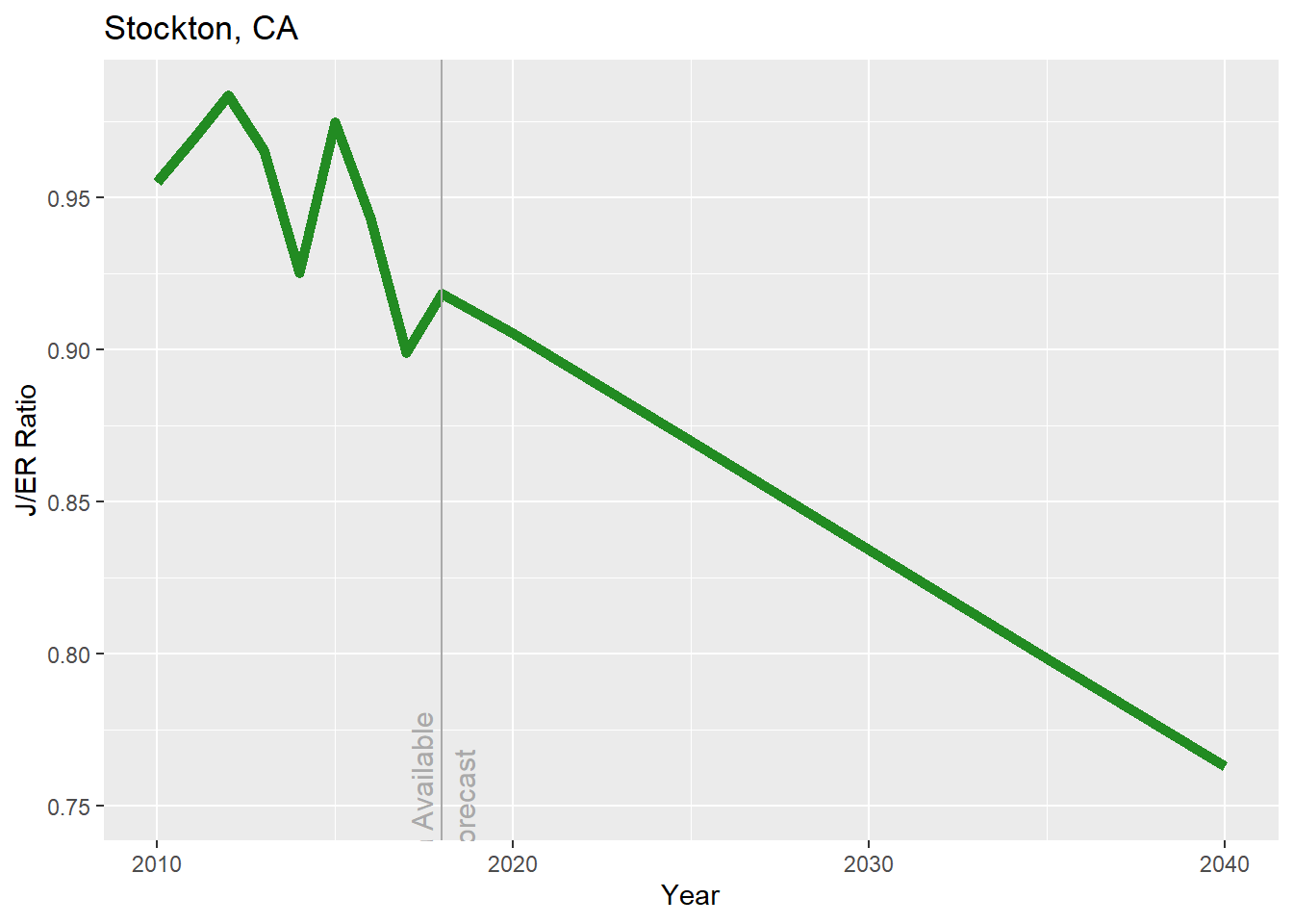
Figure 2.5: Historical jobs to employed residents ratio for Stockton 2010-2018, followed by projections to 2040.
\(~\)
ggplot(pop_jobs_stockton_w_projection, aes(x = Year)) +
  geom_line(aes(y = `Employed Residents`/100000, colour = "Employed Residents"), size = 2) +
  geom_line(aes(y = Jobs/100000, colour = "Jobs"), size = 2) +
  geom_line(aes(y = Population/100000, colour = "Population"), size = 2) +
  geom_vline(aes(xintercept = 2018), color = "dark grey") +
  annotate("text",label= "Data Available\n", color = "dark grey", x=2018, y=2, angle = 90, size=4) +
  annotate("text",label= "\nForecast", color = "dark grey", x=2018, y=2, angle = 90, size=4) +
  scale_colour_manual(values = c("purple","blue","red")) +
  labs(title = "Stockton, CA", y = "Count (100,000s)", colour = "")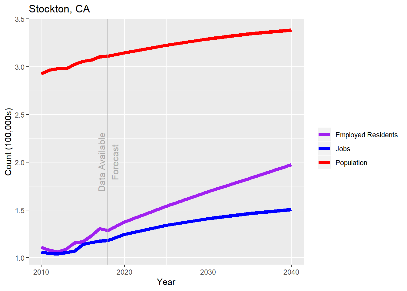
Figure 2.6: Historical population, employed residents, and jobs for Stockton 2010-2018, followed by projections to 2040.
\(~\)
Estimation of the average earnings of Stockton jobs is not possible using the QWI data from the previous section, which is only available at the County level. However, using LODES data, we can recreate a table of job counts by top-level NAICS industry sector (20 total).
# stockton_rac <-
#   2010:2017 %>%
#   map_dfr(function(year){
#     ca_rac <-
#       grab_lodes(
#         state = "ca",
#         year = year,
#         lodes_type = "rac",
#         job_type = "JT01",
#         segment = "S000",
#         state_part = "main",
#         agg_geo = "bg"
#       )
#
#     temp <-
#       stockton_bgs_full %>%
#       geo_join(ca_rac, "GEOID", "h_bg")
#
#     return(temp)
#   })
#
# save(stockton_rac, file = "C:/Users/derek/Google Drive/City Systems/Stockton Green Economy/stockton_rac.Rdata")
load("C:/Users/derek/Google Drive/City Systems/Stockton Green Economy/stockton_rac.Rdata")

jobs_stockton_residents <-
  stockton_rac %>%
  group_by(year) %>%
  summarize_at(
    vars(CNS01:CNS20),
    sum,
    na.rm=T
  ) %>%
  st_set_geometry(NULL) %>%
  gather(
    -year,
    key = "code",
    value = "Jobs"
  ) %>%
  mutate(
    industry =
      case_when(
        code == "CNS01" ~ "Agriculture, Forestry, Fishing and Hunting",
        code == "CNS02" ~ "Mining, Quarrying, and Oil and Gas Extraction",
        code == "CNS03" ~ "Utilities",
        code == "CNS04" ~ "Construction",
        code == "CNS05" ~ "Manufacturing",
        code == "CNS06" ~ "Wholesale Trade",
        code == "CNS07" ~ "Retail Trade",
        code == "CNS08" ~ "Transportation and Warehousing",
        code == "CNS09" ~ "Information",
        code == "CNS10" ~ "Finance and Insurance",
        code == "CNS11" ~ "Real Estate and Rental and Leasing",
        code == "CNS12" ~ "Professional, Scientific, and Technical Services",
        code == "CNS13" ~ "Management of Companies and Enterprises",
        code == "CNS14" ~ "Administrative and Support and Waste Management and Remediation Services",
        code == "CNS15" ~ "Educational Services",
        code == "CNS16" ~ "Health Care and Social Assistance",
        code == "CNS17" ~ "Arts, Entertainment, and Recreation",
        code == "CNS18" ~ "Accommodation and Food Services",
        code == "CNS20" ~ "Public Administration",
        code == "CNS19" ~ "Other Services"
      )
  ) %>%
  dplyr::select(-code)

jobs_stockton_residents_17 <-
  jobs_stockton_residents %>%
  filter(year == 2017) %>%
  dplyr::select(-year) %>%
  arrange(desc(Jobs)) %>%
  transmute(
    `NAICS Industry` = industry,
    Jobs = prettyNum(round(Jobs,-2),big.mark=",")
  )

kable(
  jobs_stockton_residents_17,
  booktabs = TRUE,
  caption = 'Job counts by NAICS industry sector for Stockton 2017.'
  ) %>%
  kable_styling() %>%
scroll_box(width = "100%")| NAICS Industry | Jobs |
|---|---|
| Health Care and Social Assistance | 19,600 |
| Retail Trade | 14,800 |
| Educational Services | 11,200 |
| Manufacturing | 10,800 |
| Accommodation and Food Services | 10,700 |
| Administrative and Support and Waste Management and Remediation Services | 9,200 |
| Transportation and Warehousing | 8,500 |
| Construction | 7,300 |
| Public Administration | 6,900 |
| Wholesale Trade | 6,800 |
| Agriculture, Forestry, Fishing and Hunting | 5,100 |
| Professional, Scientific, and Technical Services | 4,900 |
| Other Services | 3,800 |
| Finance and Insurance | 3,000 |
| Information | 1,800 |
| Arts, Entertainment, and Recreation | 1,700 |
| Management of Companies and Enterprises | 1,700 |
| Real Estate and Rental and Leasing | 1,500 |
| Utilities | 1,000 |
| Mining, Quarrying, and Oil and Gas Extraction | 100 |