4.2 Vehicle Emissions

4.2.1 Strategy: Electric Vehicle Program

In Section 2.7, we used EMFAC2017 to estimate the penetration of EVs into the market in a business-as-usual situation from now till 2040, reaching about 5% in 2040. Any increase beyond this percentage would contribute to a further reduction in gCO2/mile, which would reduce the overall GHG footprint of Stockton’s commute travel.

The following table shows how transportation tCO2 changes in 2040 with different EV penetration percentages. This model assumes that the distribution of vehicle types (car vs. truck, gasoline vs. diesel) does not change apart from the increase in percentage of EVs. For example, within gasoline vehicles, about 70% are projected to be cars and the rest are trucks; we do not change that assumption as we decrease the number of gasoline vehicles overall.

non_electric <-
  emfac_summary %>% 
  filter(Year == 2040) %>% 
  filter(`Fuel Type` != "Electric") %>% 
  pull(`Percent Vehicles`) %>% 
  sum()

emfac_modify <-
  c(0,5,10,15,20,25,30,35,40,45) %>% 
  map_dfr(function(x){
    temp <-
      emfac_summary %>% 
      filter(Year == 2040) %>% 
      mutate(
        `Percent Vehicles` = `Percent Vehicles`*(1-x/non_electric),
        product = `Percent Vehicles`/100*`gCO2 Running Exhaust`,
        product2 = `Percent Vehicles`/100*`gCO2 Start Exhaust`
      ) %>% 
      group_by(Year) %>% 
      summarize(
        `gCO2/mile` = sum(product),
        `gCO2/trip` = sum(product2)
      ) %>% 
      left_join(ghg_forecast_prep %>% dplyr::select(vmtperjob, `Employed Residents`, Year,Population), by = "Year") %>% 
      mutate(
        `Percent EVs` = 5.19 + x,
        `gCO2/mile` = `gCO2/mile`,
        tco2 = vmtperjob * `Employed Residents` *2*369.39*`gCO2/mile`*1.1023e-6 + `Employed Residents`*2*369.39*`gCO2/trip`*1.1023e-6 + 4100*Population*`gCO2/mile`*1.1023e-6
      )
  })

emfac_modify_table <-
  emfac_modify %>% 
  transmute(
    `Percent EVs` = paste0(round(`Percent EVs`),"%"),
    `gCO2/mile` = round(`gCO2/mile`),
    `Transportation tCO2` = prettyNum(round(tco2,-4), big.mark = ",") 
  )

kable(
  emfac_modify_table,
  booktabs = TRUE,
  caption = 'Impact of increasing EV penetration by increments of 5% on commute GHGs in 2040.'
) %>% 
  kable_styling() %>% 
  scroll_box(width = "100%")

Table 4.1: Impact of increasing EV penetration by increments of 5% on commute GHGs in 2040.

Percent EVs	gCO2/mile	Transportation tCO2
5%	256	1,670,000
10%	243	1,580,000
15%	229	1,490,000
20%	216	1,410,000
25%	202	1,320,000
30%	189	1,230,000
35%	175	1,140,000
40%	162	1,050,000
45%	148	970,000
50%	135	880,000

\(~\)

emfac_modify %>% 
  ggplot(
    aes(
      x = `Percent EVs`,
      y = `tco2`
    )
  ) +
  geom_line(size = 2, colour = "forest green") +
  labs(title = "Commute Emissions in 2040", y = "Transportation tCO2")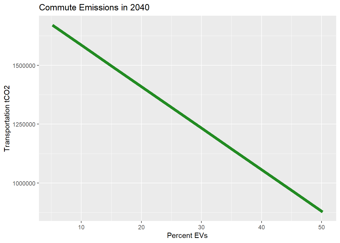

Figure 4.2: Impact of increasing EV penetration by increments of 5% on commute GHGs in 2040.

\(~\)

Note that while EVs can be effective at reducing gCO2/mile, transit strategies are even more effective because they reduce VMTs directly. Ultimately Stockton should proactively pursue strategies in both VMT reduction and vehicle emissions reduction because this sector of GHG emissions can use as many interventions as possible.