2.4 Origin-Destination Commute Analysis

As seen in the previous section, transportation is the largest single contributor of GHG emissions in Stockton, as is true for all of California. Within this sector, passenger vehicle emissions are by far the largest portion, and these are relatively easy to relate to their direct proxy, vehicle miles traveled (VMT), and normalize by drivers to understand current driving behavior. Specifically, commutes (driving to work) are the largest share of passenger vehicle emissions (other driving to/from amenities can be analyzed separately), and we can access data as recent as 2017 to understand commute patterns of Stockton residents to different job destinations inside and outside of SJC. What we find is that VMT is significant, and significantly locked in to the nature of job opportunity in faraway locations like the Bay Area. This means that VMT reduction is a crucial component in any overall green economy strategy, and it can be tackled directly through transportation strategies like public transit and EV deployment, but also indirectly by attracting high-quality jobs to Stockton, which on average will shift workers from faraway jobs to local jobs, thereby reducing VMTs. A comprehensive origin-destination commute analysis, as performed below, helps us quantify total VMTs attributable to commuting as well as model the specific impacts of different direct or indirect VMT reduction strategies.

In this section, we first examine the distribution of job locations for SJC in comparison to neighboring counties, as well as Stockton in particular. The following section will then analyze vehicle miles traveled for these commute trips.

2.4.1 County-level Analysis

Our key dataset is from Longitudinal Employer-Household Dynamics Origin-Destination Employment Statistics (LODES), which can be downloaded by state and is available up to 2017.

Some reported workplaces in LODES are as far away as Los Angeles County and are likely data errors (e.g. the company headquarters is in Los Angeles but the actual workplace is much closer, or the employee works from home). These workplaces are left in the datasets shown in this section, but are removed later when calculating VMTs.

The LODES dataset also disaggregates jobs by three age groups:

Number of jobs of workers age 29 or younger
Number of jobs for workers age 30 to 54
Number of jobs for workers age 55 or older

It also disaggregates jobs by three wage tiers:

Number of jobs with earnings $1250/month or less
Number of jobs with earnings $1251/month to $3333/month
Number of jobs with earnings greater than $3333/month

It also disaggregates jobs by three broad sectors:

Number of jobs in Goods Producing industry sectors
Number of jobs in Trade, Transportation, and Utilities industry sectors
Number of jobs in All Other Services industry sectors

The following table shows the counts of jobs in these subcategories that are held by SJC residents traveling to a workplace in SJC or its top 14 contiguous neighboring counties. The percent jobs shown are percentages of SJC employed residents; so of all SJC employed residents, 48% work within SJC.

# for(year in 2002:2017){
# 
#   ca_lodes <-
#     grab_lodes(
#       state = "ca",
#       year = year,
#       lodes_type = "od",
#       job_type = "JT01", #Primary Jobs
#       segment = "S000",
#       state_part = "main",
#       agg_geo = "tract"
#     )
# 
#   for(county in county_neighbors$COUNTYFP){
#     county_tracts <-
#       ca_tracts %>%
#       filter(COUNTYFP == county)
# 
#     county_lodes_h <-
#       ca_lodes[which(ca_lodes$h_tract %in% county_tracts$GEOID),]
# 
#     save(county_lodes_h, file = paste0("C:/Users/derek/Google Drive/City Systems/Stockton Green Economy/LODES/county_lodes_",county,"_",year,"_tract_noroute.Rdata"))
# 
#   }
# }

load("C:/Users/derek/Google Drive/City Systems/Stockton Green Economy/LODES/county_lodes_077_2017_tract_noroute.Rdata")

sjc_lodes_w_counties <- 
  county_lodes_h %>% 
  mutate(
    COUNTY = substr(w_tract,3,5)
  ) %>% 
  group_by(COUNTY) %>% 
  summarise_at(
    c("S000","SA01","SA02","SA03","SE01","SE02","SE03","SI01","SI02","SI03"), 
    sum,
    na.rm=T
  ) %>% 
  transmute(
    County = COUNTY,
    Jobs = S000,
    `Percent Jobs` = S000/sum(S000, na.rm=T),
    `Percent of jobs for workers age 29 or younger` = SA01/sum(SA01, na.rm=T),
    `Percent of jobs for workers age 30 to 54` = SA02/sum(SA02, na.rm=T),
    `Percent of jobs for workers age 55 or older` = SA03/sum(SA03, na.rm=T),
    `Percent of jobs with earnings $1250/month or less` = SE01/sum(SE01, na.rm=T),
    `Percent of jobs with earnings $1251/month to $3333/month` = SE02/sum(SE02, na.rm=T),
    `Percent of jobs with earnings greater than $3333/month` = SE03/sum(SE03, na.rm=T),
    `Percent of jobs in Goods Producing industry sectors` = SI01/sum(SI01, na.rm=T),
    `Percent of jobs in Trade, Transportation, and Utilities industry sectors` = SI02/sum(SI02, na.rm=T),
    `Percent of jobs in All Other Services industry sectors` = SI03/sum(SI03, na.rm=T)
  ) %>% 
  arrange(desc(Jobs))

sjc_lodes_w_top_counties <- 
  sjc_lodes_w_counties[1:19,] %>% 
  left_join(ca_counties %>% 
  dplyr::select(COUNTYFP, NAME), by = c("County" = "COUNTYFP")) %>% 
  dplyr::select(-County) %>%
  dplyr::select(NAME,everything()) %>% 
  rename(County = NAME) %>% 
  arrange(desc(Jobs)) %>% 
  filter(!County %in% c("Los Angeles","San Bernardino","Orange","San Diego")) %>% 
  st_as_sf()

sjc_lodes_w_top_counties_table <- 
  sjc_lodes_w_top_counties %>% 
  st_set_geometry(NULL) %>% 
  transmute(
    `County (where SJC residents work)` = County,
    `Jobs (held by SJC residents)` = prettyNum(round(Jobs,-2),big.mark=","),
    `Percent jobs (held by SJC residents)` = paste0(round(`Percent Jobs`*100),"%"),
    `Percent of jobs for workers age 29 or younger` = paste0(round(`Percent of jobs for workers age 29 or younger`*100),"%"),
    `Percent of jobs for workers age 30 to 54` = paste0(round(`Percent of jobs for workers age 30 to 54`*100),"%"),
    `Percent of jobs for workers age 55 or older` = paste0(round(`Percent of jobs for workers age 55 or older`*100),"%"),
    `Percent of jobs with earnings $1250/month or less` = paste0(round(`Percent of jobs with earnings $1250/month or less`*100),"%"),
    `Percent of jobs with earnings $1251/month to $3333/month` = paste0(round(`Percent of jobs with earnings $1251/month to $3333/month`*100),"%"),
    `Percent of jobs with earnings greater than $3333/month` = paste0(round(`Percent of jobs with earnings greater than $3333/month`*100),"%"),
    `Percent of jobs in Goods Producing industry sectors` = paste0(round(`Percent of jobs in Goods Producing industry sectors`*100),"%"),
    `Percent of jobs in Trade, Transportation, and Utilities industry sectors` = paste0(round(`Percent of jobs in Trade, Transportation, and Utilities industry sectors`*100),"%"),
    `Percent of jobs in All Other Services industry sectors` = paste0(round(`Percent of jobs in All Other Services industry sectors`*100),"%")
  )

kable(
  sjc_lodes_w_top_counties_table, 
  booktabs = TRUE, 
  caption = 'Top 15 counties where SJC residents work, including SJC. Los Angeles, San Bernardino, Orange, and San Diego Counties were removed. Data from LODES, 2017.'
  ) %>% 
  kable_styling() %>%
  scroll_box(width = "100%")

Table 2.14: Top 15 counties where SJC residents work, including SJC. Los Angeles, San Bernardino, Orange, and San Diego Counties were removed. Data from LODES, 2017.
County (where SJC residents work)	Jobs (held by SJC residents)	Percent jobs (held by SJC residents)	Percent of jobs for workers age 29 or younger	Percent of jobs for workers age 30 to 54	Percent of jobs for workers age 55 or older	Percent of jobs with earnings $1250/month or less	Percent of jobs with earnings $1251/month to $3333/month	Percent of jobs with earnings greater than $3333/month	Percent of jobs in Goods Producing industry sectors	Percent of jobs in Trade, Transportation, and Utilities industry sectors	Percent of jobs in All Other Services industry sectors
San Joaquin	127,100	48%	47%	47%	53%	54%	53%	42%	47%	46%	50%
Alameda	30,600	12%	10%	13%	10%	8%	8%	15%	15%	11%	11%
Sacramento	17,100	7%	8%	6%	6%	6%	7%	6%	4%	7%	7%
Santa Clara	16,100	6%	6%	6%	6%	4%	5%	8%	8%	6%	6%
Stanislaus	15,300	6%	6%	6%	6%	6%	6%	6%	6%	6%	6%
Contra Costa	10,300	4%	4%	4%	3%	3%	4%	4%	4%	4%	4%
San Francisco	5,900	2%	2%	2%	2%	2%	2%	3%	1%	2%	3%
San Mateo	4,800	2%	2%	2%	2%	1%	1%	2%	1%	2%	2%
Solano	3,400	1%	1%	1%	1%	1%	1%	1%	1%	2%	1%
Fresno	2,700	1%	1%	1%	1%	2%	1%	1%	1%	1%	1%
Placer	2,500	1%	1%	1%	1%	1%	1%	1%	1%	1%	1%
Yolo	1,700	1%	1%	1%	1%	1%	1%	1%	1%	1%	1%
Sonoma	1,500	1%	1%	1%	1%	1%	1%	1%	0%	1%	1%
Monterey	1,300	0%	1%	0%	1%	1%	1%	0%	1%	1%	0%
Merced	1,200	0%	1%	0%	0%	1%	1%	0%	1%	1%	0%

$~$

The following table compares SJC with neighboring counties in terms of the percentage of jobs held by its residents that are “local”, meaning within the same county. This figure mirrors Figure 2.3, which showed J/ER ratio for the same counties, all stagnating or in decline. The figure below provides one contribution, which is declining local jobs for local residents, not just for SJC but for its neighboring counties.

county_localjobs <- NULL

for(year in 2002:2017){
  for(county in county_neighbors$COUNTYFP){
    load(paste0("C:/Users/derek/Google Drive/City Systems/Stockton Green Economy/LODES/county_lodes_",county,"_",year,"_tract_noroute.Rdata"))
    
    county_lodes_w_counties <- 
      county_lodes_h %>% 
      mutate(
        COUNTY = substr(w_tract,3,5)
      ) %>%
      group_by(COUNTY) %>% 
      summarise_at(
        c("S000","SA01","SA02","SA03","SE01","SE02","SE03","SI01","SI02","SI03"), 
        sum,
        na.rm=T
      ) %>% 
      transmute(
        Year = year,
        County = COUNTY,
        Jobs = S000,
        `Percent Jobs` = S000/sum(S000, na.rm=T),
        `Percent of jobs for workers age 29 or younger` = SA01/sum(SA01, na.rm=T),
        `Percent of jobs for workers age 30 to 54` = SA02/sum(SA02, na.rm=T),
        `Percent of jobs for workers age 55 or older` = SA03/sum(SA03, na.rm=T),
        `Percent of jobs with earnings $1250/month or less` = SE01/sum(SE01, na.rm=T),
        `Percent of jobs with earnings $1251/month to $3333/month` = SE02/sum(SE02, na.rm=T),
        `Percent of jobs with earnings greater than $3333/month` = SE03/sum(SE03, na.rm=T),
        `Percent of jobs in Goods Producing industry sectors` = SI01/sum(SI01, na.rm=T),
        `Percent of jobs in Trade, Transportation, and Utilities industry sectors` = SI02/sum(SI02, na.rm=T),
        `Percent of jobs in All Other Services industry sectors` = SI03/sum(SI03, na.rm=T)
      ) %>% 
      filter(County == county) %>% 
      mutate(County = county_neighbors[which(county_neighbors$COUNTYFP == county),]$NAME)
    
    county_localjobs <-
      county_localjobs %>% 
      rbind(
        county_lodes_w_counties
      )
  }
}

county_localjobs %>% 
  filter(County %in% c("San Joaquin","Alameda","Fresno","Stanislaus","Sacramento","Contra Costa")) %>%
  ggplot(
    aes(
      x = Year,
      y = `Percent Jobs`,
      colour = County
    )
  ) +
  geom_line()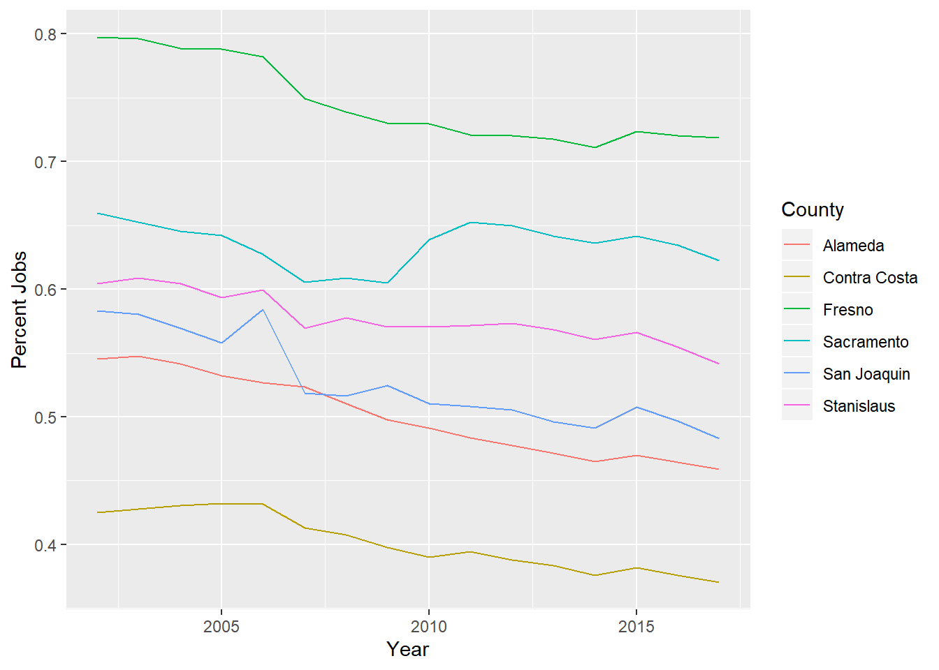

Figure 2.10: Percent of county residents who work within their home county, 2002 to 2017. Data from LODES.

$~$

2.4.2 City-level Analysis

The following table shows the counts of jobs in these subcategories for the top 15 contiguous neighboring counties to Stockton, including SJC. Note that the jobs being counted are those held by Stockton residents who are traveling to a workplace in the listed regions. 41% of Stockton employed residents work within Stockton. These jobs could be considered valuable for avoiding the “brain drain” of local talent to other places, as well as for creating the smallest transportation footprint.

# for(year in 2002:2017){
# 
#   ca_lodes <-
#     grab_lodes(
#       state = "ca",
#       year = year,
#       lodes_type = "od",
#       job_type = "JT01", #Primary Jobs
#       segment = "S000",
#       state_part = "main",
#       agg_geo = "bg"
#     )
# 
#     stockton_lodes_h <-
#       ca_lodes[which(ca_lodes$h_bg %in% stockton_bgs_full$GEOID),]
# 
#     save(stockton_lodes_h, file = paste0("C:/Users/derek/Google Drive/City Systems/Stockton Green Economy/LODES/stockton_lodes_",year,"_tract_noroute.Rdata"))
# 
# }

load("C:/Users/derek/Google Drive/City Systems/Stockton Green Economy/LODES/stockton_lodes_2017_tract_noroute.Rdata")

stockton_lodes_w_counties <- 
  stockton_lodes_h %>% 
  mutate(
    Workplace = ifelse(
      w_bg %in% stockton_bgs_full$GEOID,
      "75000",
      substr(w_bg,3,5)
    )
  ) %>% 
  group_by(Workplace) %>% 
  summarise_at(
    c("S000","SA01","SA02","SA03","SE01","SE02","SE03","SI01","SI02","SI03"), 
    sum,
    na.rm=T
  ) %>% 
  transmute(
    Workplace = Workplace,
    Jobs = S000,
    `Percent Jobs` = S000/sum(S000, na.rm=T),
    `Percent of jobs for workers age 29 or younger` = SA01/sum(SA01, na.rm=T),
    `Percent of jobs for workers age 30 to 54` = SA02/sum(SA02, na.rm=T),
    `Percent of jobs for workers age 55 or older` = SA03/sum(SA03, na.rm=T),
    `Percent of jobs with earnings $1250/month or less` = SE01/sum(SE01, na.rm=T),
    `Percent of jobs with earnings $1251/month to $3333/month` = SE02/sum(SE02, na.rm=T),
    `Percent of jobs with earnings greater than $3333/month` = SE03/sum(SE03, na.rm=T),
    `Percent of jobs in Goods Producing industry sectors` = SI01/sum(SI01, na.rm=T),
    `Percent of jobs in Trade, Transportation, and Utilities industry sectors` = SI02/sum(SI02, na.rm=T),
    `Percent of jobs in All Other Services industry sectors` = SI03/sum(SI03, na.rm=T)
  ) %>%  
  arrange(desc(Jobs))

#merge county shapefile with stockton geometry
ca_counties_and_stockton <-
  ca_counties %>% 
  dplyr::select(COUNTYFP, NAME) %>% 
  rbind(
    stockton_boundary %>% 
      mutate(
        COUNTYFP = PLACEFP
      ) %>% 
      dplyr::select(COUNTYFP, NAME)
  )

ca_counties_and_stockton[which(ca_counties_and_stockton$COUNTYFP == "077"),] <-
  st_difference(
    ca_counties_and_stockton[which(ca_counties_and_stockton$COUNTYFP == "077"),],
    ca_counties_and_stockton[which(ca_counties_and_stockton$NAME == "Stockton"),]
  ) %>% 
  dplyr::select(COUNTYFP,NAME)

ca_counties_and_stockton[which(ca_counties_and_stockton$COUNTYFP == "077"),]$NAME <-
  "San Joaquin (not including Stockton)"

stockton_lodes_w_top_counties <- 
  stockton_lodes_w_counties[1:19,] %>% 
  left_join(ca_counties_and_stockton %>% 
  dplyr::select(COUNTYFP, NAME), by = c("Workplace" = "COUNTYFP")) %>% 
  dplyr::select(-Workplace) %>%
  dplyr::select(NAME,everything()) %>% 
  rename(County = NAME) %>% 
  arrange(desc(Jobs)) %>% 
  filter(!County %in% c("Los Angeles","San Bernardino","Orange","San Diego")) %>% 
  st_as_sf()

stockton_lodes_w_top_counties_table <- 
  stockton_lodes_w_top_counties %>% 
  st_set_geometry(NULL) %>% 
  transmute(
    `Workplace (where Stockton residents work)` = County,
    `Jobs (held by Stockton residents)` = prettyNum(round(Jobs,-2),big.mark=","),
    `Percent jobs (held by Stockton residents)` = paste0(round(`Percent Jobs`*100),"%"),
    `Percent of jobs for workers age 29 or younger` = paste0(round(`Percent of jobs for workers age 29 or younger`*100),"%"),
    `Percent of jobs for workers age 30 to 54` = paste0(round(`Percent of jobs for workers age 30 to 54`*100),"%"),
    `Percent of jobs for workers age 55 or older` = paste0(round(`Percent of jobs for workers age 55 or older`*100),"%"),
    `Percent of jobs with earnings $1250/month or less` = paste0(round(`Percent of jobs with earnings $1250/month or less`*100),"%"),
    `Percent of jobs with earnings $1251/month to $3333/month` = paste0(round(`Percent of jobs with earnings $1251/month to $3333/month`*100),"%"),
    `Percent of jobs with earnings greater than $3333/month` = paste0(round(`Percent of jobs with earnings greater than $3333/month`*100),"%"),
    `Percent of jobs in Goods Producing industry sectors` = paste0(round(`Percent of jobs in Goods Producing industry sectors`*100),"%"),
    `Percent of jobs in Trade, Transportation, and Utilities industry sectors` = paste0(round(`Percent of jobs in Trade, Transportation, and Utilities industry sectors`*100),"%"),
    `Percent of jobs in All Other Services industry sectors` = paste0(round(`Percent of jobs in All Other Services industry sectors`*100),"%")
  )

kable(
  stockton_lodes_w_top_counties_table, 
  booktabs = TRUE, 
  # caption = 'Top 15 workplaces where Stockton residents work. Includes Stockton as a workplace destination separate from the rest of SJC. All other listed workplaces are counties. Los Angeles, San Bernardino, Orange, and San Diego Counties were removed. Data from LODES, 2017.'
  ) %>% 
  kable_styling() %>%
  scroll_box(width = "100%")

Workplace (where Stockton residents work)	Jobs (held by Stockton residents)	Percent jobs (held by Stockton residents)	Percent of jobs for workers age 29 or younger	Percent of jobs for workers age 30 to 54	Percent of jobs for workers age 55 or older	Percent of jobs with earnings $1250/month or less	Percent of jobs with earnings $1251/month to $3333/month	Percent of jobs with earnings greater than $3333/month	Percent of jobs in Goods Producing industry sectors	Percent of jobs in Trade, Transportation, and Utilities industry sectors	Percent of jobs in All Other Services industry sectors
Stockton	53,000	41%	37%	41%	47%	46%	41%	38%	30%	33%	48%
San Joaquin (not including Stockton)	18,600	14%	15%	14%	14%	13%	17%	12%	23%	18%	10%
Alameda	9,400	7%	7%	8%	6%	5%	6%	9%	10%	8%	6%
Sacramento	9,300	7%	8%	7%	6%	7%	7%	7%	5%	8%	8%
Santa Clara	5,900	5%	5%	4%	4%	4%	4%	5%	5%	5%	4%
Stanislaus	4,700	4%	4%	4%	3%	4%	4%	3%	4%	4%	3%
Contra Costa	4,500	3%	4%	4%	3%	3%	3%	4%	4%	3%	4%
San Francisco	3,200	2%	2%	3%	2%	2%	2%	4%	1%	2%	3%
San Mateo	2,400	2%	2%	2%	2%	1%	1%	2%	1%	2%	2%
Solano	1,700	1%	1%	1%	1%	1%	1%	2%	1%	2%	1%
Fresno	1,400	1%	1%	1%	1%	2%	1%	1%	1%	1%	1%
Placer	1,200	1%	1%	1%	1%	1%	1%	1%	1%	1%	1%
Yolo	900	1%	1%	1%	1%	1%	1%	1%	1%	1%	1%
Sonoma	800	1%	1%	1%	1%	1%	1%	1%	0%	1%	1%
Monterey	700	1%	1%	0%	1%	1%	1%	0%	1%	0%	0%

$~$

The following maps help to visualize the specific distribution of Stockton residents’ jobs in the categories of age, earnings, and industry sector.

37% of younger (under 29) Stockton employed residents work within Stockton, and another 15% work outside of Stockton but within SJC. Beyond that, there are higher concentrations of these younger workers in Sacramento and Alameda County compared to other neighboring counties.

# map <- mapview(stockton_lodes_w_top_counties[-c(1,2),c("Percent of jobs for workers age 29 or younger")], zcol = "Percent of jobs for workers age 29 or younger", map.types = c("OpenStreetMap"), legend = TRUE, layer.name = 'Percent of jobs</br>for workers age</br>29 or younger')
# 
# mapshot(map,url="map-stockton-lodes-w-top-counties-youth.html")

knitr::include_url("https://citysystems.github.io/stockton-greeneconomy/map-stockton-lodes-w-top-counties-youth.html")

Figure 2.11: Top 13 counties where Stockton residents work, not including SJC - percent of overall jobs for Stockton workers age 29 or younger located in workplace. Data from LODES, 2017.

$~$

46% of lower-wage (less than $1,250/month) Stockton employed residents work within Stockton, and another 13% work outside of Stockton but within SJC. Beyond that, there is a higher concentration of these lower-wage workers in Sacramento County compared to other neighboring counties.

# map = mapview(stockton_lodes_w_top_counties[-c(1,2),c("Percent of jobs with earnings $1250/month or less")], zcol = "Percent of jobs with earnings $1250/month or less", map.types = c("OpenStreetMap"), legend = TRUE, layer.name = 'Percent of jobs</br>with earnings</br>$1250/month or less')
# 
# mapshot(map,url="map-stockton-lodes-w-top-counties-lowinc.html")

knitr::include_url("https://citysystems.github.io/stockton-greeneconomy/map-stockton-lodes-w-top-counties-lowinc.html")

Figure 2.12: Top 13 counties where Stockton residents work, not including SJC - percent of overall jobs for Stockton workers with earnings $1250/month or less located in workplace. Data from LODES, 2017.

$~$

38% of higher-wage (greater than $3,333/month) Stockton employed residents work within Stockton, and another 12% work outside of Stockton but within SJC. Note these percentages are lower than the percentages of lower-wage jobs that remain local. Beyond that, there is a higher concentration of these high-wage workers in Alameda County compared to other neighboring counties. Perhaps targeted marketing of businesses that are providing these higher-wage jobs in Alameda County to move to Stockton could be an effective investment.

# map = mapview(stockton_lodes_w_top_counties[-c(1,2),c("Percent of jobs with earnings greater than $3333/month")], zcol = "Percent of jobs with earnings greater than $3333/month", map.types = c("OpenStreetMap"), legend = TRUE, layer.name = 'Percent of jobs</br>with earnings</br>greater than</br>$3333/month')
# 
# mapshot(map,url="map-stockton-lodes-w-top-counties-highinc.html")

knitr::include_url("https://citysystems.github.io/stockton-greeneconomy/map-stockton-lodes-w-top-counties-highinc.html")

Figure 2.13: Top 13 counties where Stockton residents work, not including SJC - percent of overall jobs for Stockton residents with earnings greater than $3333/month located in workplace. Data from LODES, 2017.

$~$

30% of Stockton employed residents in Goods Producing industry sectors work within Stockton, and another 23% (a notably high percentage) work outside of Stockton but within SJC. Beyond that, there is a higher concentration of these high-wage workers in Alameda County compared to other neighboring counties.

# map = mapview(stockton_lodes_w_top_counties[-c(1,2),c("Percent of jobs in Goods Producing industry sectors")], zcol = "Percent of jobs in Goods Producing industry sectors", map.types = c("OpenStreetMap"), legend = TRUE, layer.name = 'Percent of jobs</br>in Goods Producing</br>industry sectors')
# 
# mapshot(map,url="map-stockton-lodes-w-top-counties-goods.html")

knitr::include_url("https://citysystems.github.io/stockton-greeneconomy/map-stockton-lodes-w-top-counties-goods.html")

Figure 2.14: Top 13 counties where Stockton residents work, not including SJC - percent of jobs for Stockton residents in Goods Producing industry sectors located in workplace. Data from LODES, 2017.

$~$

33% of Stockton employed residents in Trade, Transportation, and Utilities industry sectors work within Stockton, and another 18% work outside of Stockton but within SJC. Beyond that, there are higher concentrations of these high-wage workers in Sacramento and Alameda County compared to other neighboring counties.

# # map = mapview(stockton_lodes_w_top_counties[-c(1,2),c("Percent of jobs in Trade, Transportation, and Utilities industry sectors")], zcol = "Percent of jobs in Trade, Transportation, and Utilities industry sectors", map.types = c("OpenStreetMap"), legend = TRUE, layer.name = 'Percent of jobs</br>in Trade, Transportation,</br>and Utilities</br>industry sectors')
# 
# mapshot(map,url="map-stockton-lodes-w-top-counties-trade.html")

knitr::include_url("https://citysystems.github.io/stockton-greeneconomy/map-stockton-lodes-w-top-counties-trade.html")

Figure 2.15: Top 13 counties where Stockton residents work, not including SJC - percent of jobs for Stockton residents in Trade, Transportation, and Utilities industry sectors located in workplace. Data from LODES, 2017.

$~$

48% (a notably high percentage) of Stockton employed residents in All Other Services industry sectors work within Stockton, and another 10% work outside of Stockton but within SJC. Beyond that, there is a higher concentrations of these high-wage workers in Alameda County compared to other neighboring counties.

# map = mapview(stockton_lodes_w_top_counties[-c(1,2),c("Percent of jobs in All Other Services industry sectors")], zcol = "Percent of jobs in All Other Services industry sectors", map.types = c("OpenStreetMap"), legend = TRUE, layer.name = 'Percent of jobs</br>in All Other Services</br>industry sectors')
# 
# mapshot(map,url="map-stockton-lodes-w-top-counties-services.html")

knitr::include_url("https://citysystems.github.io/stockton-greeneconomy/map-stockton-lodes-w-top-counties-services.html")

Figure 2.16: Top 13 counties where Stockton residents work, not including SJC - percent of jobs for Stockton residents in All Other Services industry sectors located in workplace. Data from LODES, 2017.

$~$

While LODES origin-destination data doesn’t provide job types at a granularity lower than the three broad industry sector categories in the previous three maps, one possible assumption to make is that the distribution of NAICS industry sectors in a destination block group, which is available through the separate Workplace Area Characteristics dataset from LODES, is the same distribution for specifically Stockton residents who work in that block group. Using this assumption, we created estimates of the locations of specific types of industries and wage levels for Stockton employed residents.

The following table summarizes the number of Stockton workers estimated in each NAICS industry, by wage level.

# ca_wac <-
#   2010:2017 %>%
#   map_dfr(function(year){
#     ca_wac <-
#       grab_lodes(
#         state = "ca",
#         year = year,
#         lodes_type = "wac",
#         job_type = "JT01",
#         segment = "S000",
#         state_part = "main",
#         agg_geo = "bg"
#       )
# 
#     return(ca_wac)
#   })
# 
# save(ca_wac, file = "C:/Users/derek/Google Drive/City Systems/Stockton Green Economy/ca_wac.Rdata")

load("C:/Users/derek/Google Drive/City Systems/Stockton Green Economy/ca_wac.Rdata")

load("C:/Users/derek/Google Drive/City Systems/Stockton Green Economy/LODES/stockton_lodes_2017_tract_noroute.Rdata")

stockton_lodes_h_join_wac <- 
  stockton_lodes_h %>% 
  dplyr::select(-c(year,state)) %>% 
  left_join(
    ca_wac %>% 
      filter(year == 2017), 
    by = "w_bg"
  )

stockton_lodes_h_join_wac_normalize <-
  stockton_lodes_h_join_wac %>% 
  mutate(
    goodsproducing = CNS01+CNS02+CNS04+CNS05,
    tradetransportutil = CNS03+CNS06+CNS07+CNS08,
    services = CNS09+CNS10+CNS11+CNS12+CNS13+CNS14+CNS15+CNS16+CNS17+CNS18+CNS19+CNS20
  ) %>% 
  mutate_at(
    .vars = vars(CNS01,CNS02,CNS04,CNS05),
    .funs = list(~ SI01*./goodsproducing)
  ) %>% 
  mutate_at(
    .vars = vars(CNS03,CNS06,CNS07,CNS08),
    .funs = list(~ SI02*./tradetransportutil)
  ) %>%
  mutate_at(
    .vars = vars(CNS09:CNS20),
    .funs = list(~ SI03*./services)
  ) %>% 
  dplyr::select(-c(SA01:SA03,C000:CE03,CR01:CFS05),SE01,SE02,SE03) %>% 
  mutate(low=SE01,mid=SE02,high=SE03) %>% 
  gather(key = "type", value, low:high) %>% 
  mutate_at(
    .vars = vars(CNS01:CNS20),
    .funs = list(~ ./S000*value)
  ) %>% 
  gather(key = "type2", value2, CNS01:CNS20) %>% 
  unite(temp,type,type2) %>% 
  spread(temp,value2) %>% 
  filter(value > 0) %>% 
  dplyr::select(-value)


stockton_naics_jobs <-
  stockton_lodes_h_join_wac_normalize %>% 
  group_by(w_bg) %>% 
  summarize_at(
    vars(S000,SE01,SE02,SE03,high_CNS01:mid_CNS20),
    sum, 
    na.rm=T
  ) %>% 
  mutate_at(
    .vars = vars(high_CNS01:mid_CNS20),
    .funs = list(~ round(.,0))
  )

stockton_naics_jobs <-
  stockton_lodes_h_join_wac_normalize %>% 
  group_by(w_bg) %>% 
  summarize_at(
    vars(S000,SE01,SE02,SE03,high_CNS01:mid_CNS20),
    sum, 
    na.rm=T
  ) %>% 
  mutate_at(
    .vars = vars(high_CNS01:mid_CNS20),
    .funs = list(~ round(.))
  )

stockton_naics_jobs_summary <-
  rbind(
    stockton_naics_jobs[,-1] %>% colSums()
  ) %>% 
  t() %>%
  as.data.frame() %>% 
  rownames_to_column() %>% 
  mutate(
    jobs = V1,
    rowname = 
      case_when(
        rowname == "SE01" ~ "low_Total",
        rowname == "SE02" ~ "mid_Total",
        rowname == "SE03" ~ "high_Total",
        TRUE ~ rowname
      )
  ) %>% 
  dplyr::select(-V1) %>% 
  filter(!rowname %in% c("S000")) %>% 
  separate(
    rowname,
    into = c("wage","industry"),
    sep = "_"
  ) %>% 
  mutate(
    industry =
      case_when(
        industry == "CNS01" ~ "Agriculture, Forestry, Fishing and Hunting",
        industry == "CNS02" ~ "Mining, Quarrying, and Oil and Gas Extraction",
        industry == "CNS03" ~ "Utilities",
        industry == "CNS04" ~ "Construction",
        industry == "CNS05" ~ "Manufacturing",
        industry == "CNS06" ~ "Wholesale Trade",
        industry == "CNS07" ~ "Retail Trade",
        industry == "CNS08" ~ "Transportation and Warehousing",
        industry == "CNS09" ~ "Information",
        industry == "CNS10" ~ "Finance and Insurance",
        industry == "CNS11" ~ "Real Estate and Rental and Leasing",
        industry == "CNS12" ~ "Professional, Scientific, and Technical Services",
        industry == "CNS13" ~ "Management of Companies and Enterprises",
        industry == "CNS14" ~ "Administrative and Support and Waste Management and Remediation Services",
        industry == "CNS15" ~ "Educational Services",
        industry == "CNS16" ~ "Health Care and Social Assistance",
        industry == "CNS17" ~ "Arts, Entertainment, and Recreation",
        industry == "CNS18" ~ "Accommodation and Food Services",
        industry == "CNS20" ~ "Public Administration",
        industry == "CNS19" ~ "Other Services",
        TRUE ~ industry
      )
  ) %>% 
  spread(wage,jobs) %>% 
  dplyr::select(
    `NAICS Industry` = industry,
    `Stockton Jobs with earnings $1250/month or less` = low,
    `Stockton Jobs with earnings $1251/month to $3333/month` = mid,
    `Stockton Jobs with earnings greater than $3333/month` = high
  )

stockton_naics_jobs_summary_table <-
  rbind(
    stockton_naics_jobs_summary[which(stockton_naics_jobs_summary$`NAICS Industry`=="Total"),],
    stockton_naics_jobs_summary[which(stockton_naics_jobs_summary$`NAICS Industry`!="Total"),]
  ) %>% 
  mutate_at(
    .vars = vars(-`NAICS Industry`),
    .funs = list(~ prettyNum(round(./10^(nchar(.)-2))*10^(nchar(.)-2),big.mark=","))
  )

kable(
  stockton_naics_jobs_summary_table, 
  booktabs = TRUE, 
  caption = 'Number of Stockton employed residents, by NAICS industry and wage tier. Data from LODES, 2017.'
  ) %>% 
  kable_styling() %>%
  scroll_box(width = "100%")

Table 2.15: Number of Stockton employed residents, by NAICS industry and wage tier. Data from LODES, 2017.
NAICS Industry	Stockton Jobs with earnings $1250/month or less	Stockton Jobs with earnings $1251/month to $3333/month	Stockton Jobs with earnings greater than $3333/month
Total	35,000	74,000	85,000
Accommodation and Food Services	2,500	3,900	2,500
Administrative and Support and Waste Management and Remediation Services	1,800	3,500	2,600
Agriculture, Forestry, Fishing and Hunting	1,300	2,200	1,400
Arts, Entertainment, and Recreation	350	600	500
Construction	840	2,500	3,900
Educational Services	2,400	4,000	5,000
Finance and Insurance	500	1,100	1,300
Health Care and Social Assistance	3,400	6,600	8,200
Information	270	580	940
Management of Companies and Enterprises	250	530	740
Manufacturing	1,100	3,900	5,600
Mining, Quarrying, and Oil and Gas Extraction	7	12	32
Other Services	740	1,300	1,100
Professional, Scientific, and Technical Services	820	1,700	2,400
Public Administration	650	1,600	5,000
Real Estate and Rental and Leasing	240	530	480
Retail Trade	3,400	6,800	4,300
Transportation and Warehousing	1,000	3,700	3,500
Utilities	70	220	760
Wholesale Trade	740	2,600	3,400

$~$

The percentages in the table below should be interpreted as the % of overall jobs held by Stockton residents of that industry sector and wage tier that are based in Stockton (the remainder being based in other counties). Particularly notable here are the low-percentage estimates of high-wage jobs in sectors generally related to the “knowledge economy”: Finance and Insurance (27%), Information (28%), and Professional, Scientific, and Technical Services (16%). Also notable is the low percentage of high-wage jobs in Construction (24%), which may include specialized building trades such as solar installation. These percentages are relative to an overall 51% of high-wage jobs being based in Stockton, which suggests that the best jobs in these notable industries are significantly underrepresented in the local economy.

stockton_naics_localjobs_summary <-
  rbind(
    stockton_naics_jobs[which(stockton_naics_jobs$w_bg %in% stockton_bgs_full$GEOID),-1] %>% colSums(),
    stockton_naics_jobs[,-1] %>% colSums()
  ) %>% 
  t() %>%
  as.data.frame() %>% 
  rownames_to_column() %>% 
  mutate(
    perc = round(V1/V2*100,0),
    rowname = 
      case_when(
        rowname == "SE01" ~ "low_Total",
        rowname == "SE02" ~ "mid_Total",
        rowname == "SE03" ~ "high_Total",
        TRUE ~ rowname
      )
  ) %>% 
  dplyr::select(-V1,-V2) %>% 
  filter(!rowname %in% c("S000")) %>% 
  separate(
    rowname,
    into = c("wage","industry"),
    sep = "_"
  ) %>% 
  mutate(
    industry =
      case_when(
        industry == "CNS01" ~ "Agriculture, Forestry, Fishing and Hunting",
        industry == "CNS02" ~ "Mining, Quarrying, and Oil and Gas Extraction",
        industry == "CNS03" ~ "Utilities",
        industry == "CNS04" ~ "Construction",
        industry == "CNS05" ~ "Manufacturing",
        industry == "CNS06" ~ "Wholesale Trade",
        industry == "CNS07" ~ "Retail Trade",
        industry == "CNS08" ~ "Transportation and Warehousing",
        industry == "CNS09" ~ "Information",
        industry == "CNS10" ~ "Finance and Insurance",
        industry == "CNS11" ~ "Real Estate and Rental and Leasing",
        industry == "CNS12" ~ "Professional, Scientific, and Technical Services",
        industry == "CNS13" ~ "Management of Companies and Enterprises",
        industry == "CNS14" ~ "Administrative and Support and Waste Management and Remediation Services",
        industry == "CNS15" ~ "Educational Services",
        industry == "CNS16" ~ "Health Care and Social Assistance",
        industry == "CNS17" ~ "Arts, Entertainment, and Recreation",
        industry == "CNS18" ~ "Accommodation and Food Services",
        industry == "CNS20" ~ "Public Administration",
        industry == "CNS19" ~ "Other Services",
        TRUE ~ industry
      )
  ) %>% 
  spread(wage,perc) %>% 
  dplyr::select(
    `NAICS Industry` = industry,
    `% Stockton Jobs in Stockton with earnings $1250/month or less` = low,
    `% Stockton Jobs in Stockton with earnings $1251/month to $3333/month` = mid,
    `% Stockton Jobs in Stockton with earnings greater than $3333/month` = high
  )

stockton_naics_localjobs_summary_table <-
  rbind(
    stockton_naics_localjobs_summary[which(stockton_naics_localjobs_summary$`NAICS Industry`=="Total"),],
    stockton_naics_localjobs_summary[which(stockton_naics_localjobs_summary$`NAICS Industry`!="Total"),]
  ) %>% 
  mutate_at(
    .vars = vars(-`NAICS Industry`),
    .funs = list(~ paste0(.,"%"))
  )

kable(
  stockton_naics_localjobs_summary_table, 
  booktabs = TRUE, 
  caption = 'Percent of Stockton employed residents working in Stockton, by NAICS industry and wage tier. Data from LODES, 2017.'
  ) %>% 
  kable_styling() %>%
  scroll_box(width = "100%")

Table 2.16: Percent of Stockton employed residents working in Stockton, by NAICS industry and wage tier. Data from LODES, 2017.
NAICS Industry	% Stockton Jobs in Stockton with earnings $1250/month or less	% Stockton Jobs in Stockton with earnings $1251/month to $3333/month	% Stockton Jobs in Stockton with earnings greater than $3333/month
Total	56%	50%	51%
Accommodation and Food Services	53%	44%	40%
Administrative and Support and Waste Management and Remediation Services	54%	51%	41%
Agriculture, Forestry, Fishing and Hunting	39%	25%	27%
Arts, Entertainment, and Recreation	51%	45%	47%
Construction	41%	34%	24%
Educational Services	66%	62%	59%
Finance and Insurance	47%	38%	27%
Health Care and Social Assistance	65%	58%	47%
Information	38%	38%	28%
Management of Companies and Enterprises	54%	46%	37%
Manufacturing	44%	38%	25%
Mining, Quarrying, and Oil and Gas Extraction	0%	0%	0%
Other Services	57%	52%	49%
Professional, Scientific, and Technical Services	39%	30%	16%
Public Administration	55%	66%	66%
Real Estate and Rental and Leasing	69%	52%	47%
Retail Trade	32%	30%	26%
Transportation and Warehousing	30%	29%	34%
Utilities	51%	58%	57%
Wholesale Trade	37%	41%	38%

$~$

The following maps highlight where some of these “underrepresented” jobs are distributed throughout the top counties where Stockton residents work.

stockton_lodes_w_counties_detail <-
  stockton_lodes_h_join_wac_normalize %>% 
  mutate(
    Workplace =
      ifelse(
        w_bg %in% stockton_bgs_full$GEOID,
        "75000",
        substr(w_bg,3,5)
      )
  ) %>% 
  group_by(Workplace) %>% 
  summarize_at(
    vars(S000,SE01,SE02,SE03,high_CNS01:mid_CNS20),
    sum, 
    na.rm=T
  ) %>% 
  mutate_at(
    .vars = vars(high_CNS01:mid_CNS20),
    .funs = list(~ round(.))
  )

stockton_lodes_w_construction_high <-
  ca_counties_and_stockton %>% 
  dplyr::select(COUNTYFP, NAME) %>% 
  left_join(stockton_lodes_w_counties, by = c("COUNTYFP" = "Workplace")) %>% 
  left_join(stockton_lodes_w_counties_detail, by = c("COUNTYFP" = "Workplace")) %>% 
  dplyr::select(-COUNTYFP) %>%
  filter(!NAME %in% c("Stockton","Los Angeles","San Bernardino","Orange","San Diego","Riverside")) %>% 
  filter(!is.na(Jobs)) %>% 
  arrange(desc(Jobs)) %>% 
  dplyr::select(
    County = NAME,
    `Number of High-wage Construction jobs` = high_CNS04
  )

# map = mapview(stockton_lodes_w_construction_high[1:10,c("Number of High-wage Construction jobs")], zcol = "Number of High-wage Construction jobs", map.types = c("OpenStreetMap"), legend = TRUE, layer.name = 'Number of</br>High-wage</br>Construction jobs')
# 
# mapshot(map,url="map-stockton-lodes-w-construction-high.html")

knitr::include_url("https://citysystems.github.io/stockton-greeneconomy/map-stockton-lodes-w-construction-high.html")

Figure 2.17: Top 10 counties where Stockton residents work, not including jobs in Stockton - number of high-wage jobs in Construction. Amount in Stockton: 900. Data from LODES, 2017.

$~$

stockton_lodes_w_scientific_high <-
  ca_counties_and_stockton %>% 
  dplyr::select(COUNTYFP, NAME) %>% 
  left_join(stockton_lodes_w_counties, by = c("COUNTYFP" = "Workplace")) %>% 
  left_join(stockton_lodes_w_counties_detail, by = c("COUNTYFP" = "Workplace")) %>% 
  dplyr::select(-COUNTYFP) %>%
  filter(!NAME %in% c("Stockton","Los Angeles","San Bernardino","Orange","San Diego","Riverside")) %>% 
  filter(!is.na(Jobs)) %>% 
  arrange(desc(Jobs)) %>% 
  dplyr::select(
    County = NAME,
    `Number of Professional, Scientific, and Technical Services jobs` = high_CNS12
  )

# map = mapview(stockton_lodes_w_scientific_high[1:10,c("Number of Professional, Scientific, and Technical Services jobs")], zcol = "Number of Professional, Scientific, and Technical Services jobs", map.types = c("OpenStreetMap"), legend = TRUE, layer.name = 'Number of</br>Professional,</br>Scientific,</br>and Technical</br>Services jobs')
# 
# mapshot(map,url="map-stockton-lodes-w-scientific-high.html")

knitr::include_url("https://citysystems.github.io/stockton-greeneconomy/map-stockton-lodes-w-scientific-high.html")

Figure 2.18: Top 10 counties where Stockton residents work, not including jobs in Stockton - number of high-wage jobs in Professional, Scientific, and Technical Services. Amount in Stockton: 400. Data from LODES, 2017.

$~$

Note that for high-wage jobs in Professional, Scientific, and Technical Services, San Joaquin County isn’t even the top employer of Stockton residents.