2.7 Vehicle Emissions
The previous two sections estimated the total VMTs due to commuting for Stockton workers from 2011 to 2017, and non-commuting travel for 2018, which can be used to forecast VMTs through 2040. While VMTs themselves are an important indicator of quality of life and economic vitality, from a GHG perspective we need to convert vehicle miles to emissions.
We followed the standard method for calculating vehicle emissions in California using the California Air Resources Board (CARB) Emission Factors (EMFAC) model. Using the EMFAC2017 model, we downloaded emissions rates data for 2013-2018, 2020, 2025, 2030, and 2040 in the San Joaquin Valley air basin. The data includes CARB’s model estimates for daily vehicles across passenger cars and trucks of different fuel types, along with emissions per mile for CO2 and other pollutants. A summary of the EMFAC data is provided below.
emfac <- read_csv("C:/Users/derek/Google Drive/City Systems/Stockton Green Economy/emfac.csv")

emfac_summary <-
  emfac %>%
  dplyr::select(
    Year = `Calendar Year`,
    `Vehicle Category`,
    `Fuel Type` = Fuel,
    Population,
    CO2_RUNEX,
    CO2_STREX
  ) %>%
  group_by(Year) %>%
  mutate(
    `Percent Vehicles` = round(Population/sum(Population)*100,2) %>% as.numeric(),
    `gCO2 Running Exhaust` = CO2_RUNEX %>% as.integer(),
    `gCO2 Start Exhaust` = CO2_STREX %>% as.integer()
  ) %>%
  ungroup() %>%
  dplyr::select(-Population, -CO2_RUNEX, -CO2_STREX) %>%
  mutate(
    `Fuel Type` =
      case_when(
        `Fuel Type` == "GAS" ~ "Gasoline",
        `Fuel Type` == "DSL" ~ "Diesel",
        TRUE ~ "Electric"
      ),
    `Vehicle Category` =
      case_when(
        `Vehicle Category` == "LDA" ~ "Passenger Car",
        TRUE ~ "Light Duty Truck"
      )
  ) %>%
  group_by(Year, `Vehicle Category`, `Fuel Type`) %>%
  summarize_all(sum)

kable(
  emfac_summary,
  booktabs = TRUE,
  caption = 'EMFAC2017 emission rates for vehicles in San Joaquin Valley, 2013 through 2040.'
) %>%
  kable_styling() %>%
scroll_box(width = "100%", height = "500px")| Year | Vehicle Category | Fuel Type | Percent Vehicles | gCO2 Running Exhaust | gCO2 Start Exhaust |
|---|---|---|---|---|---|
| 2013 | Light Duty Truck | Diesel | 0.03 | 809 | 0 |
| 2013 | Light Duty Truck | Electric | 0.01 | 0 | 0 |
| 2013 | Light Duty Truck | Gasoline | 31.52 | 817 | 177 |
| 2013 | Passenger Car | Diesel | 0.33 | 260 | 0 |
| 2013 | Passenger Car | Electric | 0.07 | 0 | 0 |
| 2013 | Passenger Car | Gasoline | 68.05 | 327 | 70 |
| 2014 | Light Duty Truck | Diesel | 0.03 | 791 | 0 |
| 2014 | Light Duty Truck | Electric | 0.00 | 0 | 0 |
| 2014 | Light Duty Truck | Gasoline | 31.32 | 801 | 173 |
| 2014 | Passenger Car | Diesel | 0.34 | 249 | 0 |
| 2014 | Passenger Car | Electric | 0.08 | 0 | 0 |
| 2014 | Passenger Car | Gasoline | 68.24 | 321 | 68 |
| 2015 | Light Duty Truck | Diesel | 0.05 | 783 | 0 |
| 2015 | Light Duty Truck | Electric | 0.00 | 0 | 0 |
| 2015 | Light Duty Truck | Gasoline | 31.16 | 789 | 170 |
| 2015 | Passenger Car | Diesel | 0.38 | 243 | 0 |
| 2015 | Passenger Car | Electric | 0.14 | 0 | 0 |
| 2015 | Passenger Car | Gasoline | 68.26 | 316 | 67 |
| 2016 | Light Duty Truck | Diesel | 0.05 | 780 | 0 |
| 2016 | Light Duty Truck | Electric | 0.01 | 0 | 0 |
| 2016 | Light Duty Truck | Gasoline | 31.03 | 770 | 165 |
| 2016 | Passenger Car | Diesel | 0.35 | 242 | 0 |
| 2016 | Passenger Car | Electric | 0.21 | 0 | 0 |
| 2016 | Passenger Car | Gasoline | 68.34 | 310 | 65 |
| 2017 | Light Duty Truck | Diesel | 0.06 | 768 | 0 |
| 2017 | Light Duty Truck | Electric | 0.03 | 0 | 0 |
| 2017 | Light Duty Truck | Gasoline | 30.70 | 751 | 161 |
| 2017 | Passenger Car | Diesel | 0.38 | 234 | 0 |
| 2017 | Passenger Car | Electric | 0.33 | 0 | 0 |
| 2017 | Passenger Car | Gasoline | 68.50 | 303 | 63 |
| 2018 | Light Duty Truck | Diesel | 0.08 | 752 | 0 |
| 2018 | Light Duty Truck | Electric | 0.05 | 0 | 0 |
| 2018 | Light Duty Truck | Gasoline | 30.37 | 729 | 156 |
| 2018 | Passenger Car | Diesel | 0.42 | 226 | 0 |
| 2018 | Passenger Car | Electric | 0.45 | 0 | 0 |
| 2018 | Passenger Car | Gasoline | 68.63 | 295 | 62 |
| 2020 | Light Duty Truck | Diesel | 0.10 | 729 | 0 |
| 2020 | Light Duty Truck | Electric | 0.11 | 0 | 0 |
| 2020 | Light Duty Truck | Gasoline | 29.73 | 686 | 147 |
| 2020 | Passenger Car | Diesel | 0.50 | 213 | 0 |
| 2020 | Passenger Car | Electric | 0.73 | 0 | 0 |
| 2020 | Passenger Car | Gasoline | 68.83 | 281 | 58 |
| 2025 | Light Duty Truck | Diesel | 0.15 | 655 | 0 |
| 2025 | Light Duty Truck | Electric | 0.42 | 0 | 0 |
| 2025 | Light Duty Truck | Gasoline | 28.54 | 584 | 125 |
| 2025 | Passenger Car | Diesel | 0.65 | 185 | 0 |
| 2025 | Passenger Car | Electric | 1.79 | 0 | 0 |
| 2025 | Passenger Car | Gasoline | 68.45 | 244 | 51 |
| 2030 | Light Duty Truck | Diesel | 0.18 | 578 | 0 |
| 2030 | Light Duty Truck | Electric | 0.74 | 0 | 0 |
| 2030 | Light Duty Truck | Gasoline | 27.95 | 512 | 109 |
| 2030 | Passenger Car | Diesel | 0.73 | 167 | 0 |
| 2030 | Passenger Car | Electric | 2.88 | 0 | 0 |
| 2030 | Passenger Car | Gasoline | 67.51 | 217 | 45 |
| 2035 | Light Duty Truck | Diesel | 0.20 | 530 | 0 |
| 2035 | Light Duty Truck | Electric | 0.97 | 0 | 0 |
| 2035 | Light Duty Truck | Gasoline | 27.69 | 472 | 99 |
| 2035 | Passenger Car | Diesel | 0.78 | 158 | 0 |
| 2035 | Passenger Car | Electric | 3.63 | 0 | 0 |
| 2035 | Passenger Car | Gasoline | 66.73 | 202 | 41 |
| 2040 | Light Duty Truck | Diesel | 0.21 | 505 | 0 |
| 2040 | Light Duty Truck | Electric | 1.12 | 0 | 0 |
| 2040 | Light Duty Truck | Gasoline | 27.62 | 452 | 93 |
| 2040 | Passenger Car | Diesel | 0.80 | 154 | 0 |
| 2040 | Passenger Car | Electric | 4.07 | 0 | 0 |
| 2040 | Passenger Car | Gasoline | 66.18 | 195 | 39 |
\(~\)
Emissions from N2O and CH4, along with emissions from other types of vehicles, were left out of this analysis.
We applied the CO2 emission rates above to our 2017 commute VMTs to estimate the total and average GHG emissions for Stockton workers commuting to each of the top 15 counties (filtering out counties further than 3 hours away). We made the following assumptions:
- Assuming that the distribution vehicle types for Stockton commuters matches the EMFAC breakdown, the average GHG emissions is about 440 g/mile running exhaust, and 93 g/trip start exhaust.
- For daily VMT, each vehicle was assumed to take 2 one-way trips.
- To convert daily VMT to annual VMT, the same annualization factor was used as ICLEI: 369.39. The factor appears to account for both expected reductions in VMT because of sick days, as well as expected increases in VMT because of chained trips.
The following table is sorted by total annual GHG from transportation.
load("C:/Users/derek/Google Drive/City Systems/Stockton Green Economy/LODES/stockton_lodes_2017.Rdata")

stockton_lodes_h_counties_ghg <-
  stockton_lodes_h_mode %>%
  st_set_geometry(NULL) %>%
  mutate(
    Workplace = ifelse(
      workplace %in% stockton_bgs_full$GEOID,
      "75000",
      substr(workplace,3,5)
    )
  ) %>%
  group_by(Workplace) %>%
  summarise_at(
    vars(jobs,person_miles,person_hours,vehicles,vmt),
    sum, na.rm=T
  ) %>%
  mutate(
    perc_jobs = jobs/sum(jobs),
    annual_vmt = vmt*2*369.39,
    annual_ghg = annual_vmt*439.462*1.1023e-6 + 2*369.39*vehicles*92.582*1.1023e-6,
    perc_ghg = annual_ghg/sum(annual_ghg),
    avg_ghg = annual_ghg/jobs
  ) %>%
  left_join(ca_counties_and_stockton %>%
  dplyr::select(COUNTYFP, NAME), by = c("Workplace" = "COUNTYFP")) %>%
  dplyr::select(-Workplace) %>%
  dplyr::select(NAME,everything()) %>%
  st_as_sf() %>%
  arrange(desc(annual_ghg))

stockton_lodes_h_counties_ghg_table <-
  stockton_lodes_h_counties_ghg[1:15,] %>%
  transmute(
    `Workplace (where Stockton residents work)` = NAME,
    `Jobs (held by Stockton residents)` = prettyNum(round(jobs,-2),big.mark=","),
    `Percent Jobs` = paste0(round(perc_jobs*100),"%"),
    `VMT (millions)` = prettyNum(round(annual_vmt/1000000),big.mark=","),
    `Total Annual GHG (tCO2e)` = prettyNum(round(annual_ghg,-3),big.mark=","),
    `Percent Annual GHG` = paste0(round(perc_ghg*100),"%"),
    `Average Annual GHG/worker (tCO2e)` = round(avg_ghg,1)
  )

kable(
  stockton_lodes_h_counties_ghg_table %>% st_set_geometry(NULL),
  booktabs = TRUE,
  caption = 'Top 15 workplaces where Stockton residents work, GHG emissions from transportation. Includes Stockton as a workplace destination separate from the rest of SJC. All other listed workplaces are counties. Los Angeles, San Bernardino, Orange, and San Diego Counties were removed. Data from LODES, 2017.'
) %>%
  kable_styling() %>%
scroll_box(width = "100%")| Workplace (where Stockton residents work) | Jobs (held by Stockton residents) | Percent Jobs | VMT (millions) | Total Annual GHG (tCO2e) | Percent Annual GHG | Average Annual GHG/worker (tCO2e) |
|---|---|---|---|---|---|---|
| Alameda | 9,100 | 8% | 304 | 148,000 | 15% | 16.2 |
| Santa Clara | 5,700 | 5% | 244 | 118,000 | 12% | 20.7 |
| Sacramento | 8,900 | 8% | 209 | 102,000 | 10% | 11.4 |
| Stockton | 51,500 | 44% | 191 | 96,000 | 10% | 1.9 |
| San Joaquin (not including Stockton) | 17,700 | 15% | 177 | 87,000 | 9% | 4.9 |
| San Francisco | 3,100 | 3% | 143 | 69,000 | 7% | 22.5 |
| Contra Costa | 4,400 | 4% | 123 | 60,000 | 6% | 13.7 |
| San Mateo | 2,300 | 2% | 105 | 51,000 | 5% | 22.2 |
| Fresno | 1,300 | 1% | 92 | 44,000 | 4% | 33.7 |
| Stanislaus | 4,500 | 4% | 76 | 37,000 | 4% | 8.2 |
| Solano | 1,600 | 1% | 53 | 26,000 | 3% | 15.6 |
| Placer | 1,200 | 1% | 42 | 21,000 | 2% | 17.7 |
| Sonoma | 700 | 1% | 40 | 20,000 | 2% | 26.9 |
| Monterey | 500 | 0% | 36 | 18,000 | 2% | 35.7 |
| Yolo | 900 | 1% | 27 | 13,000 | 1% | 15.1 |
\(~\)
According to the table above, 59% percent of Stockton residents work in San Joaquin County and collectively contribute 19% of all commute GHGs. The next 14 counties comprise another 39% of Stockton residents, but they collectively contribute 73% of all commute GHGs. This significant difference comes down to difference in average commute distance to each county, which is directly related to average GHG emissions per worker. In a later section, we will explore opportunities to stimulate local job creation so that some of these long-distance commutes can be converted into local commutes, reducing both the toll on the environment and the tolls on health and well-being for Stockton residents.
# map = mapview(stockton_lodes_h_counties_ghg[1:15,c("annual_ghg")], zcol = "annual_ghg", map.types = c("OpenStreetMap"), legend = TRUE, layer.name = 'Total Annual</br>GHG (tCO2e)')
#
# mapshot(map,url="map-ghg-map-2.html")

knitr::include_url("https://citysystems.github.io/stockton-greeneconomy/map-ghg-map-2.html")
Figure 2.29: Top 15 Counties where Stockton residents work - annual GHG emissions from driving. Data from LODES, 2017.
\(~\)
Similar to Table 2.14 and Table 2.15, the following table disaggregates annual GHG/commuter by NAICS industry and wage tier.
stockton_naics_ghg <-
  stockton_lodes_h_join_wac_normalize %>%
  left_join(stockton_lodes_h_mode %>%
  st_set_geometry(NULL), by = c("h_bg" = "residence", "w_bg" = "workplace")) %>%
  mutate(
    annual_vmt = vmt*2*369.39,
    annual_ghg = annual_vmt*439.462*1.1023e-6 + 2*369.39*vehicles*92.582*1.1023e-6
  ) %>%
  group_by(w_bg) %>%
  summarize_at(
    vars(S000,SE01,SE02,SE03,high_CNS01:mid_CNS20,annual_ghg),
    sum,
    na.rm=T
  ) %>%
  mutate(jobs = S000) %>%
  mutate_at(
    .vars = vars(S000,SE01,SE02,SE03,high_CNS01:mid_CNS20),
    .funs = list(~ .*annual_ghg/jobs)
  )

stockton_naics_ghg_summary <-
  rbind(
    stockton_naics_jobs[,-1] %>% colSums(),
    stockton_naics_ghg[,-1] %>% dplyr::select(-annual_ghg,-jobs) %>% colSums(na.rm=T)
  ) %>%
  t() %>%
  as.data.frame() %>%
  rownames_to_column() %>%
  mutate(
    ghg_per_worker = round(V2/V1,1),
    rowname =
      case_when(
        rowname == "SE01" ~ "low_Total",
        rowname == "SE02" ~ "mid_Total",
        rowname == "SE03" ~ "high_Total",
        TRUE ~ rowname
      )
  ) %>%
  dplyr::select(-V1,-V2) %>%
  filter(!rowname %in% c("S000")) %>%
  separate(
    rowname,
    into = c("wage","industry"),
    sep = "_"
  ) %>%
  mutate(
    industry =
      case_when(
        industry == "CNS01" ~ "Agriculture, Forestry, Fishing and Hunting",
        industry == "CNS02" ~ "Mining, Quarrying, and Oil and Gas Extraction",
        industry == "CNS03" ~ "Utilities",
        industry == "CNS04" ~ "Construction",
        industry == "CNS05" ~ "Manufacturing",
        industry == "CNS06" ~ "Wholesale Trade",
        industry == "CNS07" ~ "Retail Trade",
        industry == "CNS08" ~ "Transportation and Warehousing",
        industry == "CNS09" ~ "Information",
        industry == "CNS10" ~ "Finance and Insurance",
        industry == "CNS11" ~ "Real Estate and Rental and Leasing",
        industry == "CNS12" ~ "Professional, Scientific, and Technical Services",
        industry == "CNS13" ~ "Management of Companies and Enterprises",
        industry == "CNS14" ~ "Administrative and Support and Waste Management and Remediation Services",
        industry == "CNS15" ~ "Educational Services",
        industry == "CNS16" ~ "Health Care and Social Assistance",
        industry == "CNS17" ~ "Arts, Entertainment, and Recreation",
        industry == "CNS18" ~ "Accommodation and Food Services",
        industry == "CNS20" ~ "Public Administration",
        industry == "CNS19" ~ "Other Services",
        TRUE ~ industry
      )
  ) %>%
  spread(wage,ghg_per_worker) %>%
  dplyr::select(
    `NAICS Industry` = industry,
    `Annual GHG per Stockton worker with earnings $1250/month or less` = low,
    `Annual GHG per Stockton worker with earnings $1251/month to $3333/month` = mid,
    `Annual GHG per Stockton worker with earnings greater than $3333/month` = high
  )

stockton_naics_ghg_summary_table <-
  rbind(
    stockton_naics_ghg_summary[which(stockton_naics_ghg_summary$`NAICS Industry`=="Total"),],
    stockton_naics_ghg_summary[which(stockton_naics_ghg_summary$`NAICS Industry`!="Total"),]
  )

rownames(stockton_naics_ghg_summary_table) <- NULL

kable(
  stockton_naics_ghg_summary_table,
  booktabs = TRUE,
  caption = 'Annual commute tCO2e per Stockton commuter, by NAICS industry and wage tier. Data from LODES, 2017.'
  ) %>%
  kable_styling() %>%
scroll_box(width = "100%")| NAICS Industry | Annual GHG per Stockton worker with earnings $1250/month or less | Annual GHG per Stockton worker with earnings $1251/month to $3333/month | Annual GHG per Stockton worker with earnings greater than $3333/month |
|---|---|---|---|
| Total | 5.9 | 6.1 | 6.9 |
| Accommodation and Food Services | 7.1 | 7.7 | 9.1 |
| Administrative and Support and Waste Management and Remediation Services | 7.6 | 7.6 | 9.1 |
| Agriculture, Forestry, Fishing and Hunting | 6.4 | 6.4 | 7.1 |
| Arts, Entertainment, and Recreation | 8.9 | 8.6 | 10.2 |
| Construction | 7.2 | 7.5 | 10.1 |
| Educational Services | 5.3 | 5.3 | 5.8 |
| Finance and Insurance | 9.5 | 9.3 | 11.2 |
| Health Care and Social Assistance | 6.0 | 6.2 | 8.2 |
| Information | 12.4 | 11.8 | 13.5 |
| Management of Companies and Enterprises | 7.9 | 8.5 | 10.0 |
| Manufacturing | 6.7 | 6.6 | 9.4 |
| Mining, Quarrying, and Oil and Gas Extraction | 8.9 | 10.1 | 10.3 |
| Other Services | 8.9 | 8.3 | 9.9 |
| Professional, Scientific, and Technical Services | 11.8 | 12.0 | 14.1 |
| Public Administration | 6.6 | 5.4 | 5.9 |
| Real Estate and Rental and Leasing | 10.3 | 9.8 | 11.6 |
| Retail Trade | 9.8 | 9.4 | 10.5 |
| Transportation and Warehousing | 7.9 | 6.6 | 7.7 |
| Utilities | 10.2 | 7.1 | 7.6 |
| Wholesale Trade | 9.1 | 7.6 | 8.1 |
\(~\)
To conclude this section, we plotted changes in emissions per mile (just running exhaust) and the percentage of electric vehicles in San Joaquin County from 2013-2040. These projections will contribute to modeling business-as-usual GHG emissions. Later, one of our strategies will model the GHG reductions associated with even more progressive EV adoption beyond 5% by 2040.
vehicle_emissions_trend <-
  emfac_summary %>%
    mutate(
      product = `Percent Vehicles`/100*`gCO2 Running Exhaust`,
      product2 = `Percent Vehicles`/100*`gCO2 Start Exhaust`
    ) %>%
    group_by(Year) %>%
    summarize(
      `gCO2/mile` = sum(product),
      `gCO2/trip` = sum(product2)
    )

vehicle_emissions_trend %>%
  ggplot(
    aes(
      x = Year,
      y = `gCO2/mile`
    )
  )+
  geom_line(size = 2, colour = "orange") +
  labs(title = "San Joaquin Valley Air Basin", y = "gCO2/mile running exhaust")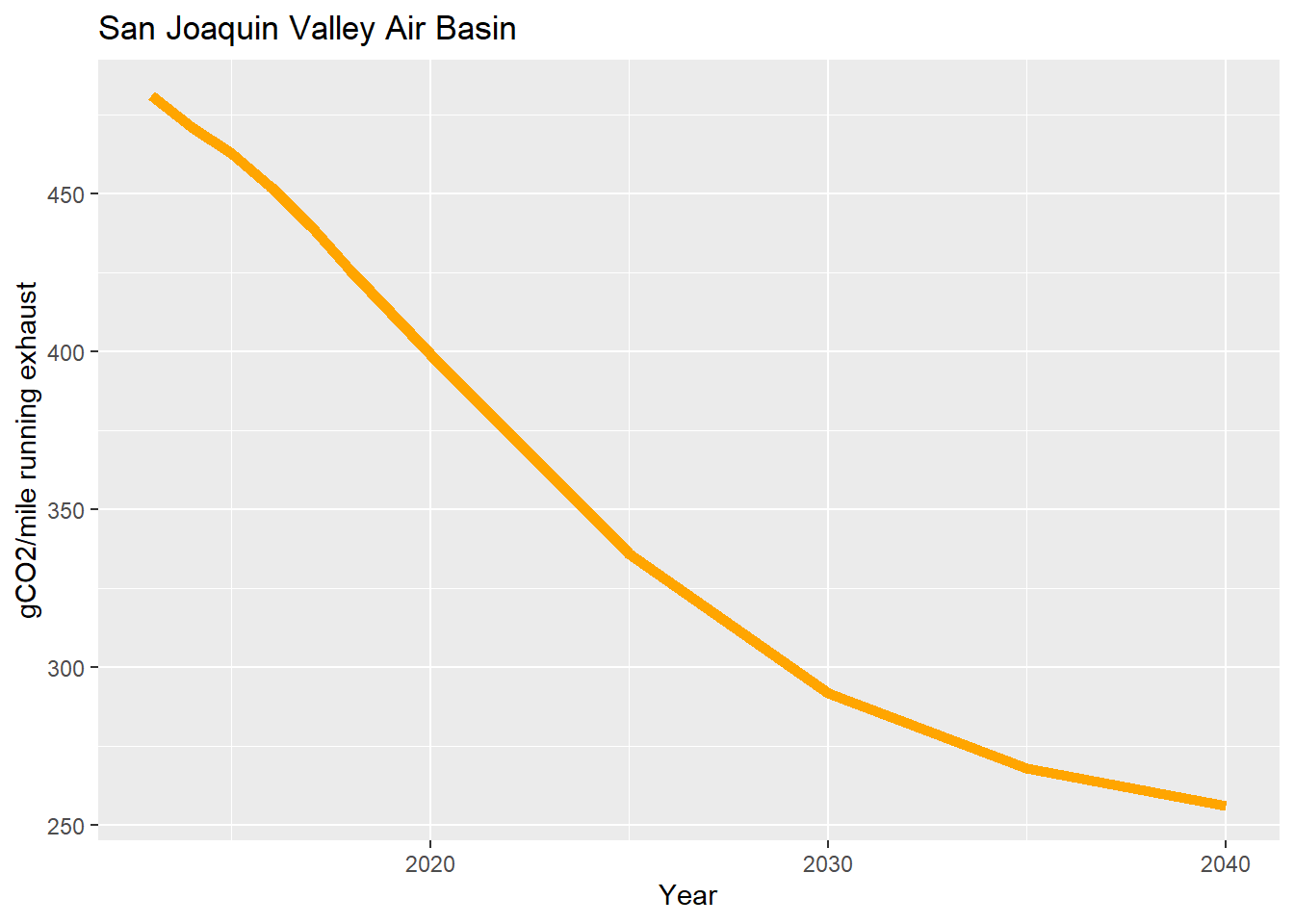
Figure 2.30: Average GHG emissions per mile for vehicles in San Joaquin Valley Air Basin, 2013-2040. Source: EMFAC2017.
\(~\)
vehicle_electric_trend <-
  emfac_summary %>%
  mutate(
    `Fuel Type` = ifelse(`Fuel Type` == "Electric", "Electric", "Other")
  ) %>%
  group_by(Year, `Fuel Type`) %>%
  summarize(count = sum(`Percent Vehicles`)) %>%
  filter(`Fuel Type` == "Electric")

vehicle_electric_trend %>%
  ggplot(
    aes(
      x = Year,
      y = `count`
    )
  )+
  geom_line(size = 2, colour = "forest green") +
  labs(title = "San Joaquin Valley Air Basin", y = "Percentage electric vehicles on road")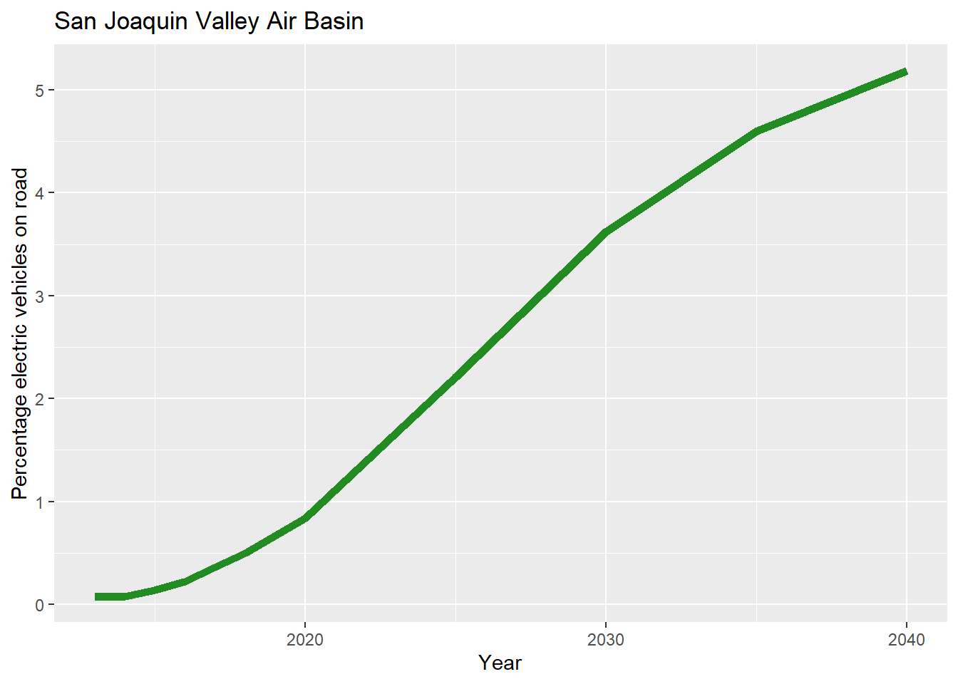
Figure 2.31: Percentage of electric vehicles in San Joaquin Valley Air Basin, 2013-2040. Source: EMFAC2017.
\(~\)
The projected busines-as-usual increase in electric vehicles on the road is a driver of the reduction in emissions/mile, namely because this electric vehicle adoption increase corresponds to a decrease in use of gasoline vehicles. However, based on a basic contribution analysis, the shift to EVs is roughly responsible for 14% of the overall gCO2/mile running exhaust reduction from 2020 to 2040 (399 to 256 gCO2/mile), while fuel efficiency improvements to gasoline vehicles is roughly responsible for 86%. This is a reminder that while EV adoption is an important driver, unless adoption can triple, improving fuel efficiency of new gasoline vehicles, retiring old vehicles, and simply reducing the amount of driving will play a greater role in reducing transportation emissions.