2.10 GHG Forecast
For our “business-as-usual” forecast of GHG emissions through 2040, and for our subsequent exploration of intervention strategies, we will focus on the following sectors for which we have used available data to refine our models: transportation, commercial energy, and residential energy. These sectors represented 58% of ICLEI’s modeled emissions in 2016. The other sectors, particularly industrial energy which comprised 24% of 2016 emissions, are also significant opportunities for GHG reductions, but are outside of the scope of this analysis without better data.
Our simplified model of transportation emissions assumes that commute one-way vehicle miles traveled per worker is on a linear trend based on recent data. Otherwise, our forecasts of growth in the number of employed residents drives changes in VMT and thus transportation emissions. Other “business-as-usual” factors, like a forecasted adoption of EVs, are not considered in this analysis.
Our simplified model of energy emissions will assume that building square footage increases with population and job growth through fixed ratios, and an underlying energy use factor for commercial and residential electricity and gas will follow the same trends as the last six years through 2040. Otherwise, a basic climate change model of heating and cooling degree days will drive additional changes in the forecasts.
In summary, the following assumptions go into inputs for the 2020-2040 forecast:
| Section | Assumption | Source/Reasoning |
|---|---|---|
| 2.1 | Population increases | Nature study by Mathew Hauer. Includes a “middle of the road” assumption for global sustainability. Population 15+ is used specifically to forecast employment. |
| 2.1 | Employment rate increases | Our choice: employment rate increases linearly based on trend from 2010-2018. |
| 2.1 | Job to employed residents ratio decreases | Our choice: J/ER ratio decreases linearly based on trend from 2010-2018. |
| 2.5 | Commute one-way VMT per worker increases | Our choice: Commute VMT/worker increases linearly based on trend from 2011-2017. |
| 2.6 | Non-commute VMT per resident stays constant | Our choice: Without trend information, we assume non-commute VMT/resident stays constant. Further analysis pending data collection is likely to reveal an upwards trend over the past few years. |
| 2.7 | GHG per vehicle mile decreases | CARB EMFAC2017 model forecasts declining emissions rates based on assumed alignment with state and federal regulations. |
| 2.7 | Electric vehicle adoption increases | CARB EMFAC2017 model forecasts increasing EV adoption based on regressions on historical data. |
| 2.8 | PG&E electricity emissions factor decreases | Our choice: We assume a linear forecast which runs from 2017’s reported factor towards a 2045 target of 100% clean energy. |
| 2.8 | Heating and cooling degree days | Cal-Adapt forecasts using the average simulation (CanESM2) under the Representative Concentration Pathway (RCP) 4.5 scenario |
| 2.8 | Energy use per capita per degree-day decreases | Our choice: combining climate, energy, and population/jobs data, we found downwards trends between 2013-2018 and assumed these trends to continue to 2040. For Commercial Gas, we leveled out the forecast at 1 kBTU/job/HDD from 2035 on. |
The table below shows the results of the various assumptions above on quantitative inputs for each year, which are used to calculate GHG emissions.
summary_TCO2E_norm_projection <-
  summary_TCO2E_norm_all

summary_TCO2E_norm_projection[7:11,1] <- c(2020,2025,2030,2035,2040)

ghg_forecast_prep <-
  summary_TCO2E_norm_projection %>%
  dplyr::select(-`Heating Degree Days`,-`Cooling Degree Days`,-Residents,-Jobs) %>%
  mutate(
    `Residential Electricity, kBTU/resident/CDD` =
      ifelse(
        Year < 2020,
        `Residential Electricity, kBTU/resident/CDD`,
        lm(
          `Residential Electricity, kBTU/resident/CDD`[1:6] ~ Year[1:6]
        )$coefficients[1]+
          lm(
            `Residential Electricity, kBTU/resident/CDD`[1:6] ~ Year[1:6]
          )$coefficients[2]*Year
      ),
    `Residential Gas, kBTU/resident/HDD` =
      ifelse(
        Year < 2020,
        `Residential Gas, kBTU/resident/HDD`,
        lm(
          `Residential Gas, kBTU/resident/HDD`[1:6] ~ Year[1:6]
        )$coefficients[1]+
          lm(
            `Residential Gas, kBTU/resident/HDD`[1:6] ~ Year[1:6]
          )$coefficients[2]*Year
      ),
    `Commercial Electricity, kBTU/job/CDD` =
      ifelse(
        Year < 2020,
        `Commercial Electricity, kBTU/job/CDD`,
        lm(
          `Commercial Electricity, kBTU/job/CDD`[1:6] ~ Year[1:6]
        )$coefficients[1]+
          lm(
            `Commercial Electricity, kBTU/job/CDD`[1:6] ~ Year[1:6]
          )$coefficients[2]*Year
      ),
    `Commercial Gas, kBTU/job/HDD` =
      ifelse(
        Year < 2020,
        `Commercial Gas, kBTU/job/HDD`,
        lm(
          `Commercial Gas, kBTU/job/HDD`[1:6] ~ Year[1:6]
        )$coefficients[1]+
          lm(
            `Commercial Gas, kBTU/job/HDD`[1:6] ~ Year[1:6]
          )$coefficients[2]*Year
      ),
    `Commercial Gas, kBTU/job/HDD` =
      ifelse(
        `Commercial Gas, kBTU/job/HDD` < 1,
        1,
        `Commercial Gas, kBTU/job/HDD`
      )
  ) %>%
  left_join(hdd, by = c("Year" = "YEAR")) %>%
  left_join(cdd, by = c("Year" = "YEAR")) %>%
  left_join(pop_jobs_stockton_w_projection %>% dplyr::select(Year, Population, `Employed Residents`, Jobs), by = "Year") %>%
  left_join(stockton_commute_vmt_tractmode %>% dplyr::select(Year, vmt, jobs_car), by = "Year") %>%
  mutate(
    vmtperjob = vmt/jobs_car
  ) %>%
  dplyr::select(-vmt,-jobs_car) %>%
  mutate(
    vmtperjob =
      ifelse(
        Year < 2018,
        vmtperjob,
        lm(
          vmtperjob[1:5] ~ Year[1:5]
        )$coefficients[1]+
          lm(
            vmtperjob[1:5] ~ Year[1:5]
          )$coefficients[2]*Year
      )
  ) %>%
  left_join(pge_elec_emissions_factor, by = c("Year" = "year")) %>%
  left_join(vehicle_emissions_trend, by = "Year") %>%
  left_join(vehicle_electric_trend, by = "Year")

ghg_forecast_table_prep <-
  ghg_forecast_prep %>%
  transmute(
    Year = Year,
    Population = prettyNum(round(Population,-3),big.mark=","),
    `Employed Residents` = prettyNum(round(`Employed Residents`,-3),big.mark=","),
    Jobs = prettyNum(round(Jobs,-3),big.mark=","),
    `One-way Commute VMT per Car-dependent Worker` = round(vmtperjob),
    `gCO2 per Vehicle Mile` = round(`gCO2/mile`),
    `Percent EVs` = count,
    `PG&E Electricity Emissions Factor` = round(factor),
    `Heating Degree Days` = hdd,
    `Cooling Degree Days` = cdd,
    `Residential Electricity, kBTU/resident/CDD` = round(`Residential Electricity, kBTU/resident/CDD`,1),
    `Residential Gas, kBTU/resident/HDD` = round(`Residential Gas, kBTU/resident/HDD`,1),
    `Commercial Electricity, kBTU/job/CDD` = round(`Commercial Electricity, kBTU/job/CDD`,1),
    `Commercial Gas, kBTU/job/HDD` = round(`Commercial Gas, kBTU/job/HDD`,1)
  )

kable(
  ghg_forecast_table_prep,
  booktabs = TRUE,
  caption = 'Input assumptions for GHG forecast to 2040.'
) %>%
  kable_styling() %>%
scroll_box(width = "100%")| Year | Population | Employed Residents | Jobs | One-way Commute VMT per Car-dependent Worker | gCO2 per Vehicle Mile | Percent EVs | PG&E Electricity Emissions Factor | Heating Degree Days | Cooling Degree Days | Residential Electricity, kBTU/resident/CDD | Residential Gas, kBTU/resident/HDD | Commercial Electricity, kBTU/job/CDD | Commercial Gas, kBTU/job/HDD |
|---|---|---|---|---|---|---|---|---|---|---|---|---|---|
| 2013 | 298,000 | 109,000 | 106,000 | 21 | 481 | 0.08 | 427 | 2090 | 2029 | 4.7 | 7.7 | 11.5 | 5.7 |
| 2014 | 302,000 | 116,000 | 107,000 | 22 | 471 | 0.08 | 435 | 2246 | 1811 | 5.2 | 5.9 | 14.1 | 4.7 |
| 2015 | 306,000 | 117,000 | 114,000 | 21 | 463 | 0.14 | 405 | 2065 | 1970 | 4.7 | 6.7 | 12.1 | 4.9 |
| 2016 | 307,000 | 123,000 | 116,000 | 22 | 452 | 0.22 | 294 | 1689 | 1700 | 5.3 | 8.0 | 13.9 | 5.0 |
| 2017 | 310,000 | 131,000 | 117,000 | 23 | 439 | 0.36 | 210 | 2244 | 1807 | 5.2 | 6.2 | 12.6 | 4.3 |
| 2018 | 311,000 | 129,000 | 118,000 | 23 | 425 | 0.50 | 202 | 2304 | 2107 | 4.1 | 6.1 | 10.5 | 4.4 |
| 2020 | 315,000 | 138,000 | 125,000 | 24 | 399 | 0.84 | 188 | 2082 | 1866 | 4.6 | 6.0 | 11.5 | 3.9 |
| 2025 | 323,000 | 154,000 | 134,000 | 25 | 336 | 2.21 | 150 | 2410 | 2106 | 4.2 | 5.2 | 10.4 | 2.8 |
| 2030 | 329,000 | 169,000 | 141,000 | 27 | 292 | 3.62 | 112 | 2087 | 2309 | 3.9 | 4.4 | 9.3 | 1.7 |
| 2035 | 335,000 | 183,000 | 146,000 | 29 | 268 | 4.60 | 75 | 2260 | 2286 | 3.5 | 3.5 | 8.2 | 1.0 |
| 2040 | 339,000 | 197,000 | 151,000 | 31 | 256 | 5.19 | 38 | 2082 | 2112 | 3.2 | 2.7 | 7.1 | 1.0 |
\(~\)
The inputs above result in the following GHG forecasts.
ghg_forecast <-
  ghg_forecast_prep %>%
  transmute(
    Year = Year,
    transport = vmtperjob * `Employed Residents` *2*369.39*`gCO2/mile`*1.1023e-6 + `Employed Residents`*2*369.39*`gCO2/trip`*1.1023e-6,
    amenity = 4100 * Population*`gCO2/mile`*1.1023e-6,
    residential = `Residential Electricity, kBTU/resident/CDD`*Population*cdd*2.9307e-7*0.000453592 + `Residential Gas, kBTU/resident/HDD`*Population*hdd/99.9761*0.00531,
    commercial = `Commercial Electricity, kBTU/job/CDD`*Jobs*cdd*2.9307e-7*0.000453592 + `Commercial Gas, kBTU/job/HDD`*Jobs*hdd/99.9761*0.00531
  )

ghg_forecast_table <-
  ghg_forecast %>%
  transmute(
    Year=Year,
    `Commute tCO2` = prettyNum(round(transport,-4),big.mark=","),
    `Non-Commute tCO2` = prettyNum(round(amenity,-3),big.mark=","),
    `Residential Building tCO2` = prettyNum(round(residential,-3),big.mark=","),
    `Commercial Building tCO2` = prettyNum(round(commercial,-3),big.mark=",")
  )

kable(
  ghg_forecast_table,
  booktabs = TRUE,
  caption = 'GHG forecast to 2040 for three subsets of GHG emissions.'
) %>%
  kable_styling() %>%
scroll_box(width = "100%")| Year | Commute tCO2 | Non-Commute tCO2 | Residential Building tCO2 | Commercial Building tCO2 |
|---|---|---|---|---|
| 2013 | 910,000 | 648,000 | 255,000 | 67,000 |
| 2014 | 980,000 | 644,000 | 213,000 | 60,000 |
| 2015 | 930,000 | 639,000 | 225,000 | 61,000 |
| 2016 | 980,000 | 627,000 | 220,000 | 52,000 |
| 2017 | 1,080,000 | 617,000 | 229,000 | 60,000 |
| 2018 | 1,030,000 | 598,000 | 232,000 | 64,000 |
| 2020 | 1,060,000 | 567,000 | 209,000 | 53,000 |
| 2025 | 1,080,000 | 490,000 | 214,000 | 48,000 |
| 2030 | 1,100,000 | 434,000 | 159,000 | 26,000 |
| 2035 | 1,170,000 | 405,000 | 142,000 | 18,000 |
| 2040 | 1,280,000 | 392,000 | 101,000 | 17,000 |
\(~\)
ghg_forecast %>%
  gather(-Year, key = "Sector", value = "tCO2") %>%
  mutate(
    Sector = case_when(
      Sector == "transport" ~ "Commute Transportation",
      Sector == "amenity" ~ "Non-commute Transportation",
      Sector == "residential" ~ "Residential Building",
      TRUE ~ "Commercial Building"
    ),
    Sector = factor(Sector, levels = c("Commercial Building","Residential Building","Non-commute Transportation", "Commute Transportation"))
  ) %>%
  ggplot(
    aes(
      x = Year,
      y = tCO2,
      fill = Sector
    )
  ) +
  geom_area()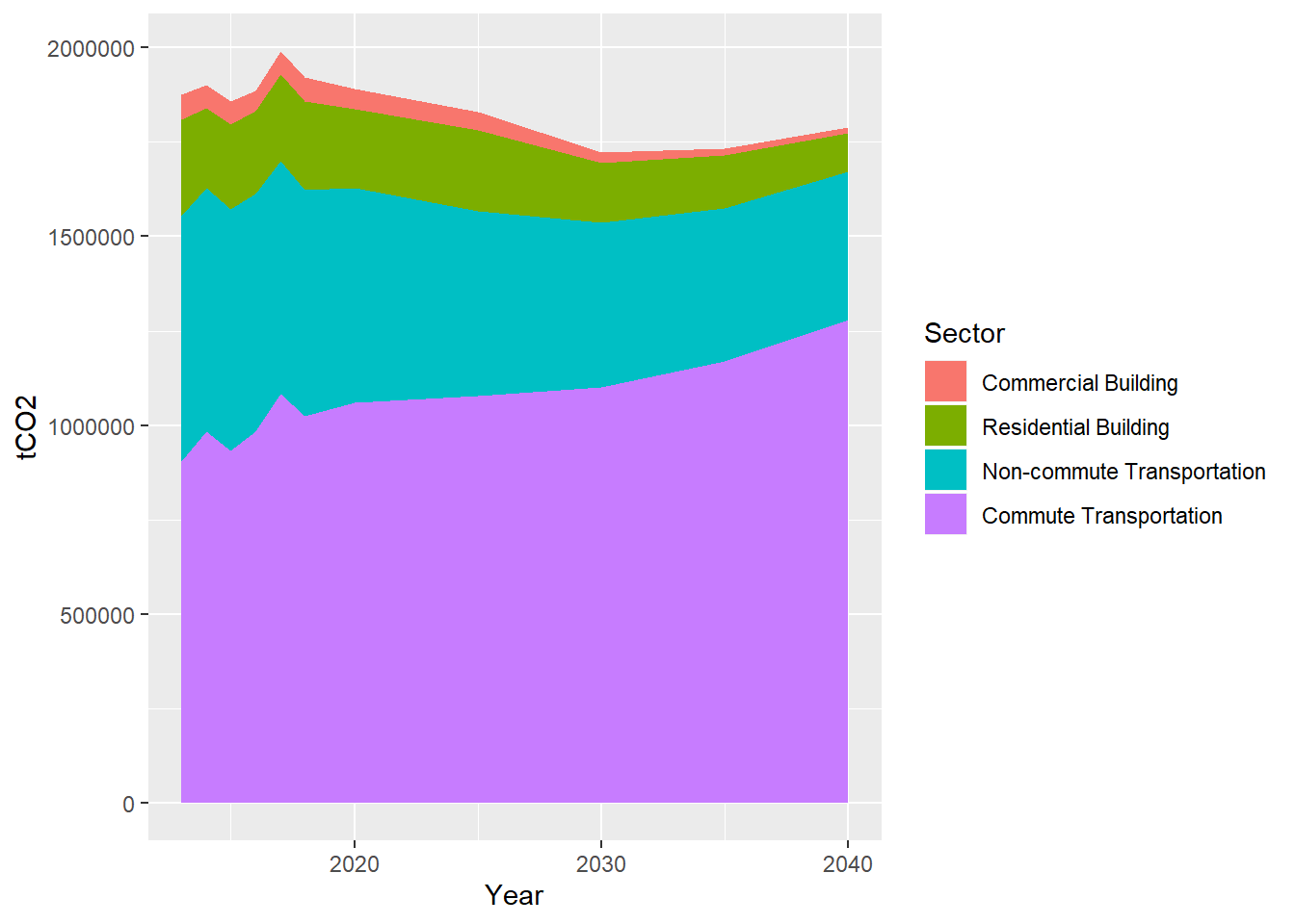
Figure 2.42: GHG forecast to 2040 for three subsets of GHG emissions.
\(~\)
The general insight is that transportation emissions are expected to increase while building emissions are expected to decrease, such that transportation emissions is even greater relative to buiding emissions than it is today.
Many differences in inputs exist between this analysis and ICLEI’s 2016 GHG Inventory, including the following:
- ICLEI’s VMT data came from a source that was only available at the SJC level and was scaled down to Stockton by population, whereas our VMT data is based on the routed distance of LODES origin-destinations. The difference these methods results in is significant (2.5 billion vs. 1.5 billion annual VMTs) and should be investigated in further work. Our Transportation tCO2 number is only for passenger commuters, whereas ICLEI’s number includes many other modes.
- ICLEI’s electricity and gas data was obtained directly from PG&E, while ours was downloaded at the zip code level from their public data portal. Since our zip codes include many parcels outside of the Stockton city boundary, it’s likely our consumption is for a larger population. As for commercial energy, ICLEI’s commercial data was combined with industrial data, while ours is separated, so that could explain why our commercial consumption numbers our lower.
The assumptions built into these forecasts are necessarily simplistic given the scope of this analysis. In particular, linear trendlines should be refined into nonlinear functions given a better understanding of growth limits for each of the domains. It’s also worth noting that some trends based on the past few years, like the desirable decline in building emissions, may be heavily influenced by active strategic policymaking, the kind which this report is meant to guide for the future. That means that “business-as-usual” is not necessarily “doing nothing” but “successfully continuing to implement progressive policies” (e.g. PG&E successfully meeting its aggressive decarbonization strategies).